Summary
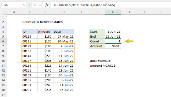
To count the number of cells that contain values between two numbers, you can use the COUNTIFS function. In the generic form of the formula (above), range represents a range of cells that contain numbers, A1 represents the lower boundary, and B1 represents the upper boundary of the numbers you want to count. In the example shown, the formula in G5, copied down, is:
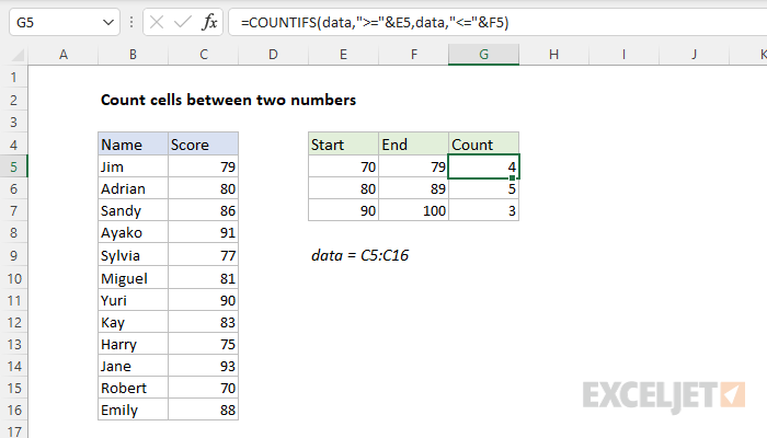
=COUNTIFS(data,">="&E5,data,"<="&F5)
where data is the named range C5:C16. As the formula is copied down, it returns a count for each of the number ranges shown in columns E and F.
Generic formula
=COUNTIFS(range,">="&A1,range,"<"&B1)
Explanation
In this example, the goal is to count numbers that fall within specific ranges. The lower value comes from the "Start" column, and the upper value comes from the "End" column. For each range, we want to include both the lower value and the upper value. For convenience, the numbers being counted are in the named range data (C5:C16). This problem can be solved with both the COUNTIFS function and the SUMPRODUCT function, as explained below.
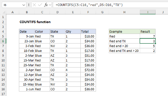
COUNTIFS function
In the example shown, the formula used to solve this problem is based on the COUNTIFS function, which is designed to count cells that meet multiple criteria. The formula in cell G5, copied down, is:
=COUNTIFS(data,">="&E5,data,"<="&F5)
COUNTIFS accepts criteria in range/criteria pairs. The first range/criteria pair checks for values in data that are greater than or equal to (>=) the "Start" value in column E:
data,">="&E5
The second range/criteria pair checks for values in data that are less than or equal to (<=) the "End" value in column F:
data,"<="&F5
Because we supply the same range (data) for both criteria, each cell in data must meet both conditions in order to be included in the final count. Note in both cases, we need to concatenate the cell reference to the logical operator. This is a quirk of RACON functions in Excel, which use a different syntax than other formulas.
As the formula is copied down column G, it returns the count of numbers that fall in the range defined by columns E and F.
SUMPRODUCT alternative
Another option for solving this problem is the SUMPRODUCT function with a formula like this:
=SUMPRODUCT((data>=E5)*(data<=F5))
This is an example of using Boolean logic. Because there are 12 values in the named range data, each logical expression inside SUMPRODUCT generates an array that contains 12 TRUE and FALSE values. The expression:
data>=E5
returns:
{TRUE;TRUE;TRUE;TRUE;TRUE;TRUE;TRUE;TRUE;TRUE;TRUE;TRUE;TRUE}
And the expression:
data<=F5
returns:
{TRUE;FALSE;FALSE;FALSE;TRUE;FALSE;FALSE;FALSE;TRUE;FALSE;TRUE;FALSE}
When these two arrays are multiplied together, the math operation causes TRUE values to be coerced to 1 and FALSE values to be coerced to zero. The result is a single array of 1s and 0s like this:
=SUMPRODUCT({1;0;0;0;1;0;0;0;1;0;1;0})
Each 1 corresponds to a number in data that meets both conditions and each 0 represents a number that fails at least one condition. With only a single array to process, SUMPRODUCT returns the sum of the numbers in the array, 4, as a final result.
Video: Boolean logic in Excel
Benefits of standard syntax
The nice thing about SUMPRODUCT is that it will handle array operations natively (no need to enter with control + shift + enter) and will accept the more standard syntax for logical expressions seen above. The standard syntax is more useful in other modern formulas. For example you could use the same exact logic with the FILTER function to return the actual numbers that meet these same conditions:
=FILTER(data,(data>=E5)*(data<=F5))
Becomes:
=FILTER(data,{1;0;0;0;1;0;0;0;1;0;1;0})
And FILTER returns the numbers greater than or equal to 70 and less than or equal to 79:
{79;77;75;70}