Explanation
In this example the goal is to parse feet and inches out in the text strings shown in column B, and create a single numeric value for total inches. The challenge is that each of the two numbers is embedded in text. The formula can be divided into two parts. In the first part of the formula, feet are extracted and converted to inches. In the second part, inches are extracted and added to the result.
Extracting feet
To extract feet and convert them to inches, we use the following snippet:
=LEFT(B5,FIND("'",B5)-1)*12
Working from the inside out, the FIND function is used to locate the position of the single quote (') in the string:
FIND("'",B5) // returns 2
We then subtract 1 (-1) and feed the result into the LEFT function as the number of characters to extract from the left:
LEFT(B5,1) // returns "8"
For cell B5, LEFT returns "8," which is then multiplied by 12 to get 96 inches. Note that the LEFT function will return a text value, but the math operation of multiplying by 12 will automatically convert the text to a number.
Extracting inches
In the second part of the formula, we extract the value for inches from the text with this snippet:
SUBSTITUTE(MID(B5,FIND("'",B5)+1,LEN(B5)),"""","")
Here we again locate the position of the single quote (') in the string with FIND. This time, however, we add 1 (+1) so that we start extracting after the single quote:
FIND("'",B5)+1 // returns 3
The result is 3, which we feed into the MID function as the start number:
MID(B5,3,LEN(B5))
For the number of characters to extract, we cheat and use the LEN function. LEN will return the total characters in B5 (5), which is a larger number of characters than remain in the string. However, MID will simply extract all remaining characters without complaint:
MID(B5,3,5) // returns " 4"""
For B5, MID will return " 4""", which goes into the SUBSTITUTE function as text:
SUBSTITUTE(" 4""","""","") // returns " 4"
The SUBSTITUTE function is configured to replace the double quote (") character with an empty string (""). In B5, SUBSTITUTE returns " 4" as text. As before, the math operation of addition will convert text value (with a space) to a number automatically, and the formula in B5 will give a final result of 100. However, to guard against a hyphen, we hand off the number returned by SUBSTITUTE to the ABS function for reasons explained below.
Note: the use of four quote characters ("""") to refer to a single double quote character (") is somewhat confusing. In brief, the outer quotes indicate a text value, the second quote is an escape character, and the third quote is the actual value. More details here.
Handling the hyphen
The measurements in B12:B13, include a hyphen (-) between feet and inches. When a hyphen is present between feet and inches, it will cause Excel to interpret the inch value as a negative number and create an incorrect result, since inches will be subtracted instead of added. To guard against this problem, we hand off the number extracted for inches to the ABS function. For example, in B12, SUBSTITUTE returns "-3 1/2" and ABS returns 3.5:
ABS("-3 1/2") // returns 3.5
Using the ABS function this way allows the same formula to handle both cases. If a hyphen is present, ABS interprets the value as negative and flips the value to a positive number. If a hyphen is not present, ABS returns the number unchanged. ABS also coerces the text value to a number.
Other units
Once you have a numeric measurement in inches, you can use the CONVERT function to convert to other units of measure.


