Convert expense time units

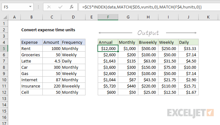
To convert an expense in one time unit (i.e. daily, weekly, monthly, etc.) to other time units, you can use a two-way INDEX and MATCH formula. In the example shown, the formula in E5 (copied across and down) is :

=$C5*INDEX(data,MATCH($D5,vunits,0),MATCH(F$4,hunits,0))

This formula uses a lookup table with named ranges as shown below:

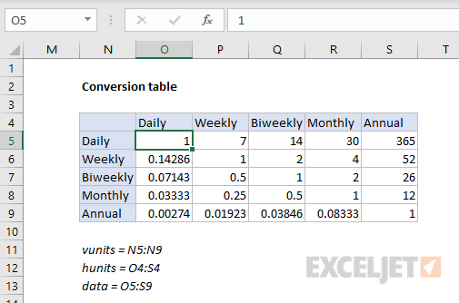
Named ranges: data (O5:S9), vunits (N5:N9), and hunits (O4:S4).

Introduction

The goal is to convert an expense in one time unit, to an equivalent expense in other time units. For example, if we have a monthly expense of $30, we want to calculate an annual expense of $360, a weekly expense of $7.50, etc.

Like so many challenges in Excel, much depends on how you approach the problem. You might first be tempted to consider a chain of nested IF formulas. This can be done, but you'll end up with a long and complicated formula.

A cleaner approach is to build a lookup table that contains conversion factors for all possible conversions, then use a two-way INDEX and MATCH formula to retrieve the required value for a given conversion. Once you have the value, you can simply multiply by the original amount.

The conversion table

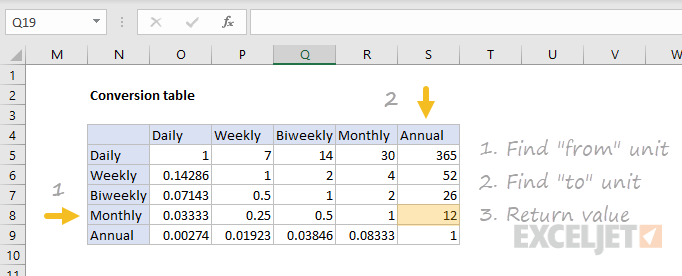
The conversion table has the same values for both vertical and horizontal labels: daily, weekly, biweekly, monthly, and annual. The "from" units are listed vertically, and the "to" units are listed horizontally. For the purposes of this example, we want to match the row first, then the column. So, if we want to convert a monthly expense to an annual expense, we match the "monthly" row, and the "annual" column, and return 12.

To populate the table itself, we use a mix of simple formulas and constants:

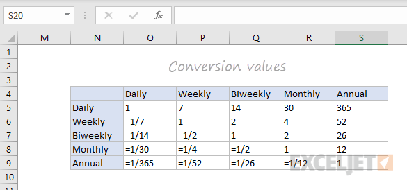
Note: Customize conversion values to meet your specific needs. Entering a value as =1/7 is an easy way to avoid entering long decimal values.

The lookup formula

Since we need to locate a conversion value based on two inputs, a "from" time unit and a "to" time unit, we need a two-way lookup formula. INDEX and MATCH provides a nice solution.  In the example shown, the formula in E5 is:

=$C5*INDEX(data,MATCH($D5,vunits,0),MATCH(F$4,hunits,0))

Working from the inside out, the first MATCH function locates the correct row:

MATCH($D5,vunits,0) // find row, returns 4

We pull the original "from" time unit from column D, which we use to find the right row in the named range vunits (N5:N9). Note $D5 is a mixed reference with the column locked, so the formula can be copied across. 

The second MATCH function locates the column:

MATCH(F$4,hunits,0) // find column, returns 5

Here, we get the lookup value from the column header in row 4, and use this to find the right "to" column in the named range hunits (O4:S4). Again, note F$4 is a mixed reference with the row locked, so the formula can be copied down. 

After both MATCH formulas return results to INDEX, we have:

=$C5*INDEX(data,4,5)

The array provided to INDEX is the named range data, (O5:S9). With a row of 4 and column of 5, INDEX returns 12, so we get a final result of 12000 like this:

=$C5*INDEX(data,4,5)
=1000*12
=12000