
Explanation
This example is based on the formula explained in detail here:
=ROW()-INDEX(ROW(data),1,1)+1>ROWS(data)-n
The formula uses the greater than operator (>) to check row in the data. On the left, the formula calculates a "current row", normalized to begin at the number 1:
=ROW()-INDEX(ROW(data),1,1)+1 // calculate current row
On the right, the formula generates a threshold number:
ROWS(data)-n // calculate threshold
When the current row is greater than the threshold, the formula returns TRUE, triggering the conditional formatting.
Conditional formatting rule
The conditional formatting rule is set up to use a formula like this:

With a table
You can't use a table name in a CF formula at present. However, you can select or enter the table data range when creating the formula in the CF window, and Excel will keep the reference up to date as the table expands or shrinks.
Related formulas

Conditional formatting based on another cell
Excel contains many built-in "presets" for highlighting values with conditional formatting, including a preset to highlight cells greater than a specific value. However, by using your own formula, you have more flexibility and control. In this example, a conditional formatting rule is set up to...

Highlight values between
When you use a formula to apply conditional formatting, the formula is evaluated for each cell in the range, relative to the active cell in the selection at the time the rule is created. So, in this case, if you apply the rule to B4:G11, with B4 as the active cell, the rule is evaluated for each of...

Highlight values greater than
When you use a formula to apply conditional formatting, the formula is evaluated relative to the active cell in the selection at the time the rule is created. So, in this case the formula =B4>100 is evaluated for each of the 40 cells in B4:G11. Because B4 is entered as a relative address, the...

Highlight cells that contain
When you use a formula to apply conditional formatting, the formula is evaluated relative to the active cell in the selection at the time the rule is created. In this case, the rule is evaluated for each of the 10 cells in B2:B11, and B2 will change to the address of the cell being evaluated each...

Highlight entire rows
When you use a formula to apply conditional formatting, the formula is evaluated relative to the active cell in the selection at the time the rule is created. In this case, the address of the active cell (B5) is used for the row (5) and entered as a mixed address , with column D locked and the row...
Related videos

How to apply conditional formatting with a formula
In this video, we'll look at how to use a formula to apply conditional formatting. Formulas allow you to make powerful and flexible conditional formatting rules that highlight just the data you want. Let's take a look. Excel provides a large number of conditional formatting presets, but there are...

Conditional formatting based on a different cell
In this video, we'll look at how to apply conditional formatting to one cell based on values in another, using a formula. Let's take a look. The easiest way to apply conditional formatting is to apply rules directly to the cells you want to format. For example, if I want to highlight the average...

How to build a search box with conditional formatting
In this video, we'll look at a way to create a search box that highlights rows in a table, by using conditional formatting, and a formula that checks several columns at once. This is a great alternative to filtering, because you can see the information you're looking for highlighted in context. Let...

How to highlight rows with conditional formatting
Using conditional formatting, It's easy to highlight cells that match a certain condition. However, it's a little trickier to highlight entire rows in a list that contains multiple columns. In this video, we'll show you how to use a formula with conditional formatting to highlight an entire row in...
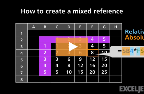
How to create a mixed reference
So what's a mixed reference? A mixed reference is a reference that's part relative and part absolute. Let's take a look. So, we've looked at both relative and absolute references, and also at a situation where we needed to use both at the same time. These are sometimes called "mixed references." A...


