Explanation
In this example, the goal is to join two one-dimensional ranges together horizontally. This can be done with the CHOOSE function and array constant.
The CHOOSE function
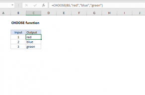
The CHOOSE function is used to select arbitrary values by numeric position. CHOOSE is a flexible function and accepts a list of text values, numbers, cell references, in any combination. For example, if we have the colors "red", "blue", and "green", we can use CHOOSE like this:
=CHOOSE(1,"red", "blue", "green") // returns "red"
=CHOOSE(2,"red", "blue", "green") // returns "blue"
=CHOOSE(3,"red", "blue", "green") // returns "green"
If we give CHOOSE an array constant like {1,2}, CHOOSE will return the first and second values in an array at the same time:
=CHOOSE({1,2}},"red", "blue", "green") // returns {"red","blue"}
The result is an array that contains two values and, in the dynamic array version of Excel, these values spill onto the worksheet into the range G5:H16.
Applications
Traditionally, the use of CHOOSE function to combine ranges is used up in tricky array formulas. The formulas below are good examples:
In these formulas, the CHOOSE function is used to create a new table (in memory) that can be used by the VLOOKUP function to workaround a difficult problem.
Note: the forthcoming HSTACK function will make this use of CHOOSE unnecessary.


