=IFS(test1, value1, [test2/value2], ...)- test1 - First logical test.
- value1 - Result when test1 is TRUE.
- test2/value2 - [optional] Second test/value pair.
Using the IFS function
The IFS function evaluates multiple logical tests and returns the value that corresponds to the first TRUE result. You can use IFS when you want a self-contained formula that tests several conditions at the same time, without nesting multiple IF functions. Formulas based on IFS are shorter and easier to read and write than the equivalent nested IF formula, because each condition and its result appear as a simple pair, and there is only one set of parentheses to manage.
Conditions are provided to IFS as test/value pairs, and IFS can handle up to 127 pairs. Each test is a logical test that returns TRUE or FALSE, and the value that follows is returned when the test is TRUE. When more than one test returns TRUE, IFS returns the value for the first TRUE result, so the order of the conditions matters. IFS does not have a built-in default value. If no test returns TRUE, IFS returns the #N/A error. The standard workaround is to enter TRUE as a final test, followed by the value to use as a default. This is explained in Return a default value below.
The IFS function is available in Excel 2019 and later, including Excel 365. In older versions of Excel, use a nested IF function instead. See 19 tips for nested IF formulas for an overview.
Key features
- Tests up to 127 condition/value pairs in a single formula
- Returns the value for the first test that returns TRUE, so order matters
- Has no built-in default value; returns #N/A when no test is TRUE
- To provide a default value, enter TRUE as a final test
- Each test is a logical expression, so operators like >, <, and = work, as do AND and OR
- Can return text, numbers, or the result of another formula
- Works with arrays and will spill results in Excel 2021+ and Excel 365
- Does not short-circuit; every test and value is evaluated
Table of contents
- Basic examples
- Assign grades from low to high
- Unit price by quantity
- Return a default value
- Handling errors
- IFS with AND and OR
- IFS with arrays
- When a lookup table is better
- IFS and performance
- IFS versus SWITCH
- Notes
Basic examples
An IFS formula with three tests can be visualized like this:
=IFS(
test1,value1, // pair 1
test2,value2, // pair 2
test3,value3 // pair 3
)
IFS evaluates the tests in order and returns the value that follows the first test that returns TRUE. For better readability, you can add line breaks to an IFS formula as shown above.
In the examples below, A1 contains the value to test. To assign a rating based on a score in A1, where 3 or greater is "Good", 2 to 3 is "Average", and anything below 2 is "Poor", you can use IFS like this:
=IFS(A1>=3,"Good",A1>=2,"Average",A1<2,"Poor") // 2.5 returns "Average"
Notice the tests are arranged to check higher values first. A score of 2.5 fails the first test but passes the second, so IFS returns "Average". IFS can also return numbers. To assign a discount rate based on an order quantity in A1:
=IFS(A1>=100,0.2,A1>=50,0.1,TRUE,0) // 75 returns 0.1
The final TRUE test above acts as a default. Without it, IFS returns #N/A for any quantity below 50. To translate a status code in A1 into a message, you can test for equality:
=IFS(A1=100,"OK",A1=200,"Warning",A1=300,"Error") // 400 returns #N/A
=IFS(A1=100,"OK",A1=200,"Warning",A1=300,"Error",TRUE,"Invalid") // 400 returns "Invalid"
With a single test/value pair, IFS behaves like an IF function with no value_if_false. However, unlike IF, the IFS function returns #N/A instead of FALSE:
=IFS(A1>10,"High") // returns "High" or #N/A
=IFS(A1>10,"High",TRUE,"Low") // returns "High" or "Low"
Assign grades from low to high
In the worksheet below, the goal is to assign a letter grade to each score in column C, using the thresholds shown in the table in F5:G9. This is the classic problem that IFS was designed to solve. The formula in D5, copied down, is:
=IFS(C5<60,"F",C5<70,"D",C5<80,"C",C5<90,"B",C5>=90,"A")
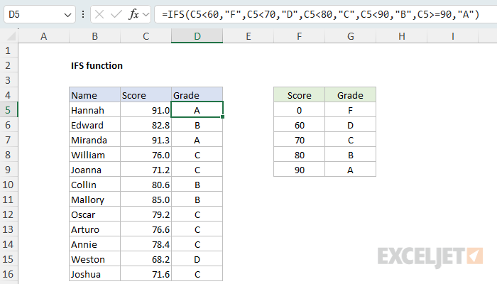
The tests are entered in order from the lowest score to the highest. IFS evaluates each test in turn and returns the grade that follows the first test that returns TRUE. For the score 76 in C8, the first two tests return FALSE (76 is not less than 60 or 70), the third test returns TRUE (76 is less than 80), and IFS returns "C". The order is what makes the formula work: because IFS stops at the first TRUE result, each test only needs to check the upper limit for its grade, since lower scores have already been handled by an earlier test.
For comparison, here is the same logic written as a nested IF formula:
=IF(C5<60,"F",IF(C5<70,"D",IF(C5<80,"C",IF(C5<90,"B","A"))))
Both formulas return the same results. However, the nested version needs four IF functions and four closing parentheses, and each new condition adds another level of nesting. The IFS version has one set of parentheses and reads as a simple list of conditions and results. For a full walkthrough of the nested version, see Nested IF function example.
Note that the final test, C5>=90, is not strictly necessary. Any score that fails all four earlier tests must be 90 or greater, so this last test is always TRUE by the time IFS reaches it. Many people write the final test explicitly to make the formula self-documenting. The alternative is to use TRUE as the final test, as described in Return a default value below. Either way, be aware of what happens with unexpected input: an empty cell evaluates as zero and returns "F", and a text value returns "A", because Excel treats text as greater than any number when comparing values.
Unit price by quantity
IFS can return numbers as well as text, which makes it useful for pricing and rate calculations. In the worksheet below, the goal is to calculate a unit price based on the quantity in column C, using the price breaks shown in the table in G5:H8: 1 to 19 units cost $7.00 each, 20 to 49 cost $6.00, 50 to 99 cost $5.00, and 100 or more cost $4.00. The formula in D5, copied down, is:
=IFS(C5>=100,4,C5>=50,5,C5>=20,6,TRUE,7)
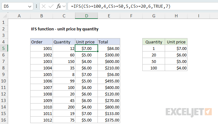
This time the tests run from the highest quantity to the lowest. A quantity of 60 fails the first test (60 is not 100 or greater) but passes the second (60 is 50 or greater), so IFS returns 5. The final TRUE test catches every quantity below 20 and returns the base price of $7.00. Because IFS returns a number, the result can be used directly in another calculation. The total in E5 is simply:
=C5*D5
The direction of the tests (low to high, or high to low) is a matter of choice, but you must pick one direction and stick with it. If the tests above were entered in random order, a quantity of 150 might be matched by C5>=20 before C5>=100 was ever checked, and the wrong price would be returned.
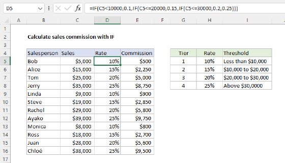
The price breaks in this example are simple, non-cumulative tiers: the whole order gets one price. For pricing where each tier applies only to the units in that tier, see Tiered discounts based on quantity. For the same pattern with commission rates, see Calculate sales commission with IF.
Return a default value
Unlike the IF function, which has a value_if_false argument, the IFS function has no built-in way to return a default value when all tests are FALSE. When no test returns TRUE, IFS returns the #N/A error. In the worksheet below, the goal is to translate the status codes in column C into messages: 100 is "OK", 200 is "Warning", and 300 is "Error". The formula in D5, copied down, is:
=IFS(C5=100,"OK",C5=200,"Warning",C5=300,"Error")
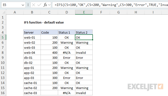
This works for the codes 100, 200, and 300. However, the code 400 in C8 does not match any test, so the formula returns #N/A. To handle this case, enter TRUE as a final test, followed by the value you want to return as a default. In this case, we classify unknown codes as "Invalid" by making that the default value. The formula in E5, copied down, is:
=IFS(C5=100,"OK",C5=200,"Warning",C5=300,"Error",TRUE,"Invalid")
Now the unrecognized code in C8 returns "Invalid" instead of #N/A. This works because IFS returns the value for the first TRUE test. The final test is always TRUE, but it is only reached when every test before it has returned FALSE, so it acts as a catch-all. Note that TRUE also catches empty cells: when C5 is blank, none of the equality tests return TRUE, and IFS returns "Invalid". If you want to return an empty string instead of a message, use TRUE followed by "". For a function that provides a default value natively, see IFS versus SWITCH below.
Handling errors
If a logical test returns an error, IFS returns that error, just as the IF function would. The tests that follow cannot "save" the result, not even a final TRUE test. The fix is to trap the error inside the test that can fail, so that a failed test becomes FALSE and IFS moves on to the next test:
=IFS(
test1,value1,
test2,value2,
IFERROR(test3,FALSE),value3,
TRUE,"all tests failed")
This most often comes up when a test contains a lookup. In the worksheet below, each ticket has a code in column C, and the limit for each code is in the table in G5:H9. The formula in D5 uses XLOOKUP to get the limit and returns "High" when the limit is over 100:
=IFS(C5="","Empty",XLOOKUP(C5,$G$5:$G$9,$H$5:$H$9)>100,"High",TRUE,"Normal")
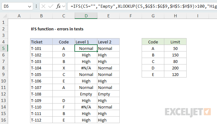
The codes in C8 and C14 are not in the table, so XLOOKUP returns #N/A, the second test becomes #N/A, and IFS returns #N/A. This looks like the "no test returned TRUE" error described above, but the cause is different, and the final TRUE test does not help. The formula in E5 wraps the lookup test in IFERROR, so an unknown code is treated as FALSE and falls through to the default "Normal":
=IFS(C5="","Empty",IFERROR(XLOOKUP(C5,$G$5:$G$9,$H$5:$H$9)>100,FALSE),"High",TRUE,"Normal")
When the lookup function has its own way to handle a missing value, like XLOOKUP's if_not_found argument, you can use that instead.
You could also wrap the entire IFS formula in IFERROR, but that hides every other error too, including the #N/A that IFS returns when no test is TRUE, so it is better to trap the error at its source.
IFS with AND and OR
Each test in IFS is a logical expression, so a test can combine more than one condition with the AND function or the OR function. In the worksheet below, the goal is to assign a shipping method to each order based on the weight in column C and whether the order is marked as rush in column D. Rush orders over 20 pounds ship "Air freight", orders that are rush or over 20 pounds ship "Priority", and everything else ships "Ground". The formula in E5, copied down, is:
=IFS(AND(D5="Yes",C5>20),"Air freight",OR(D5="Yes",C5>20),"Priority",TRUE,"Ground")
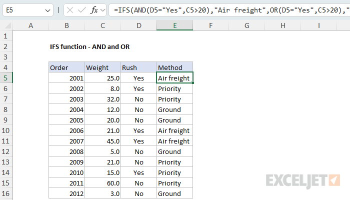
The first test uses AND to check that both conditions are true. The second test uses OR to check if either condition is true. The final TRUE test returns "Ground" for orders that are neither rush nor heavy. The order of the tests is important here as well. Any order that passes the AND test would also pass the OR test, so the more specific AND test must come first. If the OR test came first, every rush order would be assigned "Priority" and "Air freight" would never be returned.
You can also express AND and OR logic with Boolean logic, using multiplication (*) for AND and addition (+) for OR. The formula below is equivalent, since the math operations coerce TRUE and FALSE to 1 and 0, and IFS treats any non-zero number as TRUE:
=IFS((D5="Yes")*(C5>20),"Air freight",(D5="Yes")+(C5>20),"Priority",TRUE,"Ground")
The Boolean-math form has one practical advantage: it keeps working when the tests are arrays, which AND and OR do not (see IFS with arrays below). For a nested IF formula that handles a similar problem, see Nested IF with multiple AND.
IFS with arrays
In Excel 2021+ and Excel 365, the IFS function works with arrays. If a logical test returns an array of TRUE and FALSE values, IFS evaluates the tests element by element and returns an array of results, which then spills onto the worksheet. This means a single IFS formula can assign grades to an entire column of scores. In the worksheet below, the formula in D5 is:
=IFS(C5:C16<60,"F",C5:C16<70,"D",C5:C16<80,"C",C5:C16<90,"B",TRUE,"A")
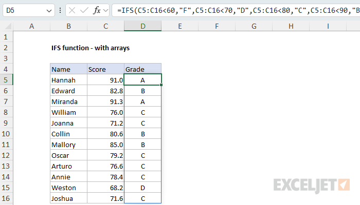
The results spill into the range D5:D16. Each test compares all twelve scores in C5:C16 at once and returns an array of twelve TRUE and FALSE values. IFS then works through the tests one row at a time, and for each row returns the value for the first TRUE result. The final TRUE test is a single value, but Excel automatically extends it to match the size of the other arrays, so it acts as a default for every row. Because one formula creates all of the results, there is no need to copy the formula down. If the scores come from an Excel Table column or a spill range reference like C5#, the results will resize automatically when the data changes.
Note that IFS will not spill if you build tests with the AND or OR functions, because they aggregate an array of TRUE and FALSE values to a single result. This behavior applies to any array formula meant to return multiple values. To apply AND or OR logic across an array, use Boolean logic instead, multiplying for AND and adding for OR, as shown in the Boolean-math formula in IFS with AND and OR above. For a walkthrough, see Array formulas with AND and OR logic.
When a lookup table is better
IFS is a good choice when there are a handful of conditions and the thresholds are stable. As the number of conditions grows, or when the thresholds need to change regularly, it is usually better to move the threshold data into a table on the worksheet and use a lookup function instead of IFS. This results in a shorter formula and keeps the thresholds visible and easy to edit in one location. In the worksheet below, the grades problem from above is solved with the XLOOKUP function in approximate match mode. The formula in D5, copied down, is:
=XLOOKUP(C5,$F$5:$F$9,$G$5:$G$9,,-1)
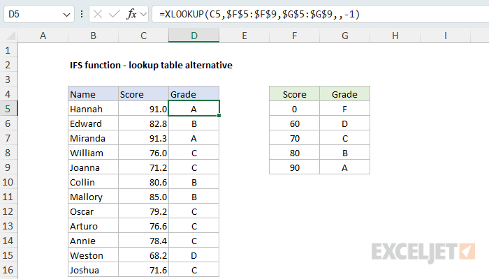
The table in F5:G9 lists the lowest score for each grade, sorted in ascending order. Setting match_mode to -1 tells XLOOKUP to find an exact match or the next smallest value. For the score 76, there is no exact match, so XLOOKUP falls back to 70, the largest threshold that is less than 76, and returns "C". This is the same "bucketing" behavior that IFS provides, without any conditions in the formula. The VLOOKUP function in approximate match mode can do the same job in any version of Excel.
For more details, see XLOOKUP basic approximate match and VLOOKUP calculate grades.
IFS and performance
You might expect the IFS function to "short-circuit" and stop evaluating once it finds a test that returns TRUE, but this is not the case. IFS evaluates all tests and all values in the formula, even when the first test is TRUE. For most formulas this makes no practical difference. However, when the values in an IFS formula involve complex or time-consuming calculations, those calculations run whether or not their test is TRUE, and this can degrade performance. It can also cause problems in recursive LAMBDA functions, because the branch that should end the recursion is evaluated even when it should be bypassed, which can trigger unintended recursion and a #NUM! error.
For a demonstration with a recursive LAMBDA, see Excel IFS short circuit evaluation on Microsoft Q&A.
To avoid these issues, consider rewriting the formula with nested IF functions or using the CHOOSE function. Both IF and CHOOSE perform true short-circuit evaluation, skipping unnecessary calculations once a result has been determined.
IFS versus SWITCH
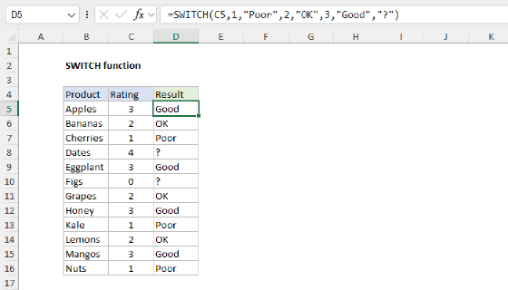
Like the SWITCH function, the IFS function lets you test more than one condition in a single self-contained formula, and both functions make it easier to write (and read) a formula with many conditions. The difference is in how the tests are written. IFS requires a separate logical test for each condition, so you can use logical operators like greater than (>) and less than (<) as needed. SWITCH compares one expression against a list of values, so the expression appears just once, but SWITCH is limited to exact matching. SWITCH also accepts a default value as its last argument, while IFS requires the TRUE workaround described above. For example, to translate a status code in A1 into a message with a default, the two functions look like this:
=IFS(A1=100,"OK",A1=200,"Warning",A1=300,"Error",TRUE,"Invalid")
=SWITCH(A1,100,"OK",200,"Warning",300,"Error","Invalid")
As a rule of thumb, use SWITCH when you are matching one value against a list of specific values, and use IFS when the conditions involve comparisons or different expressions. It is possible to use SWITCH with comparisons by matching against TRUE, as explained on the SWITCH function page, but in that case IFS is usually the more straightforward option.
Notes
- IFS returns the value for the first test that returns TRUE, so the order of the conditions matters.
- IFS does not have a built-in default value. If no test returns TRUE, IFS returns the #N/A error.
- To provide a default value, enter TRUE as a final test, followed by the value to return.
- Each test should be an expression that returns TRUE or FALSE.
- If a test returns text, IFS will return the #VALUE! error.
- If a test returns an error, IFS returns that error, unless an earlier test has already returned TRUE. See Handling errors.
- IFS can handle up to 127 test/value pairs.
- IFS does not short-circuit; all tests and values are evaluated.
- IFS is available in Excel 2019 and later. In earlier versions, use a nested IF formula.