
Summary
INDEX and MATCH is the most popular tool in Excel for performing more advanced lookups. This is because INDEX and MATCH are incredibly flexible – you can do horizontal and vertical lookups, 2-way lookups, left lookups, case-sensitive lookups, and even lookups based on multiple criteria. If you want to improve your Excel skills, INDEX and MATCH should be on your list. See below for many examples.
This article explains in simple terms how to use INDEX and MATCH together to perform lookups. It takes a step-by-step approach, first explaining INDEX, then MATCH, then showing you how to combine the two functions together to create a dynamic two-way lookup. There are more advanced examples further down the page.
Table of Contents
- The INDEX Function
- The MATCH function
- INDEX and MATCH together
- Two-way lookup with INDEX and MATCH
- Left lookup with INDEX and MATCH
- INDEX and MATCH with multiple criteria
- Case-sensitive lookup
- Finding the closest match
- INDEX and XMATCH
- More examples
The INDEX Function
The INDEX function in Excel is fantastically flexible and powerful, and you'll find it in a huge number of Excel formulas, especially advanced formulas. But what does INDEX actually do? In a nutshell, INDEX retrieves the value at a given location in a range. For example, let's say you have a table of planets in our solar system (see below), and you want to get the name of the 4th planet, Mars, with a formula. You can use INDEX like this:
=INDEX(B3:B11,4)
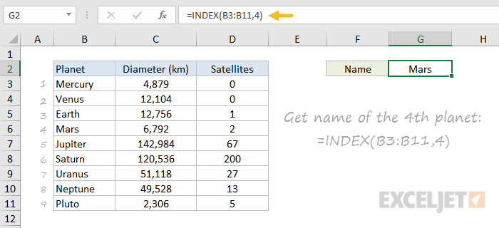
INDEX returns the value in the 4th row of the range.
Video: How to look things up with INDEX
What if you want to get the diameter of Mars with INDEX? In that case, we can supply both a row number and a column number, and provide a larger range. The INDEX formula below uses the full range of data in B3:D11, with a row number of 4 and column number of 2:
=INDEX(B3:D11,4,2)
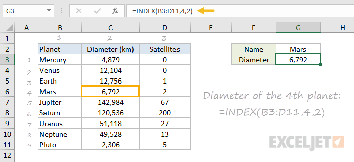
INDEX retrieves the value at row 4, column 2.
To summarize, INDEX gets a value at a given location in a range of cells based on numeric position. When the range is one-dimensional, you only need to supply a row number. When the range is two-dimensional, you'll need to supply both the row and column numbers.
At this point, you may be thinking "So what? How often do you actually know the position of something in a spreadsheet?"
Exactly right. We need a way to locate the position of things we're looking for.
Enter the MATCH function.
The MATCH function
The MATCH function is designed for one purpose: find the position of an item in a range. For example, we can use MATCH to get the position of the word "peach" in this list of fruits like this:
=MATCH("peach",B3:B9,0)
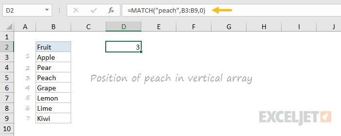
MATCH returns 3, since "Peach" is the 3rd item. MATCH is not case-sensitive.
MATCH doesn't care if a range is horizontal or vertical, as you can see below:
=MATCH("peach",C4:I4,0)
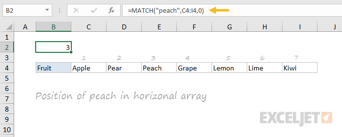
Same result with a horizontal range, MATCH returns 3.
Video: How to use MATCH for exact matches
Important: The last argument in the MATCH function is match_type. Match_type is important and controls whether matching is exact or approximate. In many cases, you will want to use zero (0) to force exact match behavior. Match_type defaults to 1, which means approximate match, so it's important to provide a value. See the MATCH page for more details.
INDEX and MATCH together
Now that we've covered the basics of INDEX and MATCH, how do we combine the two functions in a single formula? Consider the data below, a table showing a list of salespeople and monthly sales numbers for three months: January, February, and March.
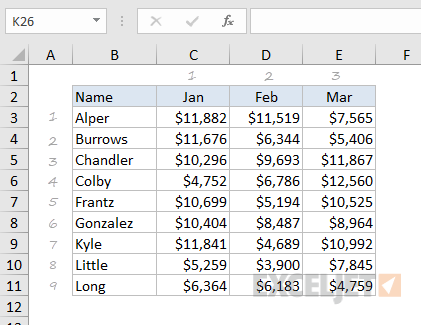
Let's say we want to write a formula that returns the sales number for February for a given salesperson. From the discussion above, we know we can give INDEX a row and column number to retrieve a value. For example, to return the February sales number for Frantz, we provide the range C3:E11 with a row 5 and column 2:
=INDEX(C3:E11,5,2) // returns $5194
But we obviously don't want to hardcode numbers. Instead, we want a dynamic lookup.
How will we do that? The MATCH function of course. MATCH will work perfectly for finding the positions we need. Working one step at a time, let's leave the column hardcoded as 2 and make the row number dynamic. Here's the revised formula, with the MATCH function nested inside INDEX in place of 5:
=INDEX(C3:E11,MATCH("Frantz",B3:B11,0),2)
Taking things one step further, we'll use the value from H2 in MATCH:
=INDEX(C3:E11,MATCH(H2,B3:B11,0),2)
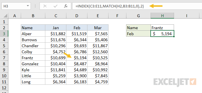
MATCH finds "Frantz" and returns 5 to INDEX for row.
To summarize:
- INDEX needs numeric positions.
- MATCH finds those positions.
- MATCH is nested inside INDEX.
Let's now tackle the column number.
Two-way lookup with INDEX and MATCH
Above, we used the MATCH function to find the row number dynamically, but we hardcoded the column number. How can we make the formula fully dynamic so we can return sales for any given salesperson in any given month? The trick is to use MATCH twice – once to get a row position, and once to get a column position.
From the examples above, we know MATCH works fine with both horizontal and vertical arrays. That means we can easily find the position of a given month with MATCH. For example, this formula returns the position of March, which is 3:
=MATCH("Mar",C2:E2,0) // returns 3
But of course, we don't want to hardcode any values, so let's update the worksheet to allow the input of a month name, and use MATCH to find the column number we need. The screen below shows the result:
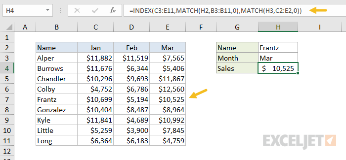
A fully dynamic, two-way lookup with INDEX and MATCH.
=INDEX(C3:E11,MATCH(H2,B3:B11,0),MATCH(H3,C2:E2,0))
The first MATCH formula returns 5 to INDEX as the row number, and the second MATCH formula returns 3 to INDEX as the column number. Once MATCH runs, the formula simplifies to:
=INDEX(C3:E11,5,3)
and INDEX correctly returns $10,525, the sales number for Frantz in March.
Note: you could use Data Validation to create dropdown menus to select salesperson and month.
Video: How to do a two-way lookup with INDEX and MATCH
Video: How to debug a formula with F9 (to see MATCH return values)
Left lookup
One of the key advantages of INDEX and MATCH over the VLOOKUP function is the ability to perform a "left lookup". Simply put, this just means a lookup where the ID column is to the right of the values you want to retrieve, as seen in the example below:
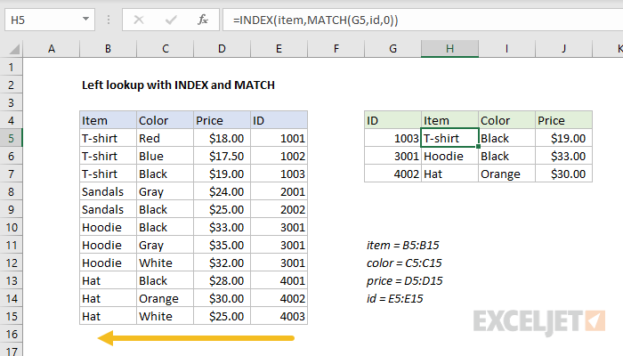
Read a detailed explanation here.
Index and Match with multiple criteria
One of the trickiest problems in Excel is a lookup based on multiple criteria. In other words, a lookup that matches on more than one column at the same time. A nice way to handle these problems is to use Boolean logic, a technique for handling TRUE and FALSE values like 1s and 0s. You can see this approach below, where we are using INDEX and MATCH and Boolean logic to find a price based on three values: Item, Color, and Size:
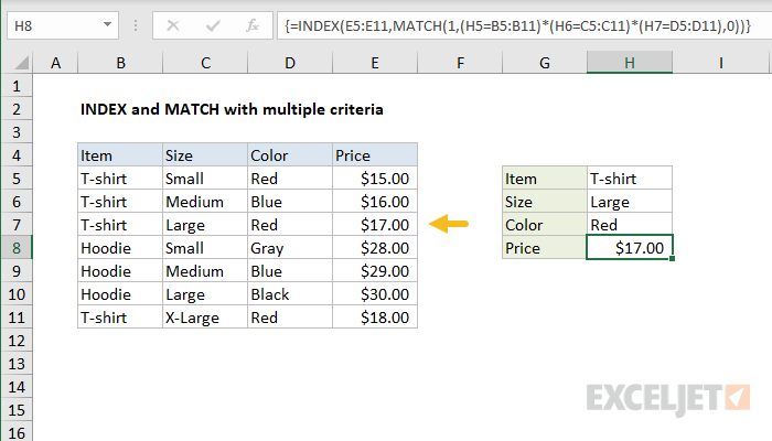
Read a detailed explanation here. You can use this same approach with XLOOKUP.
Note: this is an array formula and must be entered with control + shift + enter in Excel 2019 and older.
For a quick introduction to Booleans in Excel, see these videos from our Dynamic Array Formulas course:
One benefit of INDEX and MATCH formulas is that they use numeric indexing. This makes it easy to customize behavior to match specific data patterns. For example, you can use a step-based formula to jump directly to relevant data.
Case-sensitive lookup
By itself, the MATCH function is not case-sensitive. However, you use the EXACT function with INDEX and MATCH to perform a lookup that respects upper and lower case, as shown below:
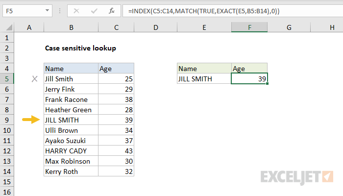
Read a detailed explanation here.
Note: this is an array formula and must be entered with control + shift + enter in Excel 2019 and older.
Closest match
Another example that shows off the flexibility of INDEX and MATCH is the problem of finding the closest match. In the example below, we use the MIN function together with the ABS function to create a lookup value and a lookup array inside the MATCH function. Essentially, we use MATCH to find the smallest difference. Then, we use INDEX to retrieve the associated trip from column B.
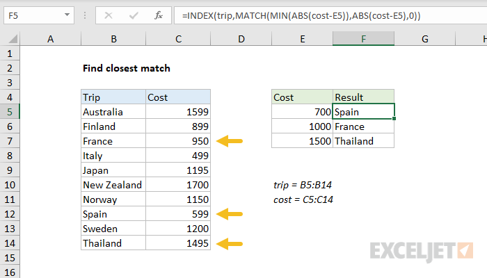
Read a detailed explanation here.
Note: this is an array formula and must be entered with control + shift + enter in Excel 2019 and older.
INDEX and XMATCH
The current version of Excel includes the XMATCH function, which is an upgraded replacement for the MATCH function. Like the MATCH function, XMATCH performs a lookup and returns a numeric position. Also like MATCH, XMATCH can perform lookups in vertical or horizontal ranges, supports both approximate and exact matches, and allows wildcards (* ?) for partial matches. But XMATCH adds even more features. The 5 key differences between XMATCH and MATCH are as follows:
- XMATCH defaults to an exact match, while MATCH defaults to an approximate match.
- XMATCH can find the next larger item or the next smaller item.
- XMATCH can perform a reverse search (i.e. search from last to first).
- XMATCH does not require values to be sorted when performing an approximate match.
- XMATCH can perform a binary search, which is specifically optimized for speed.
- XMATCH can perform a regex match, a powerful way to match complex text patterns.
So, can you simply use XMATCH in an INDEX and MATCH formula instead of MATCH? Yes, absolutely. Using XMATCH instead of the MATCH function "upgrades" the formula to include the benefits listed above.
Using XMATCH instead of the MATCH function "upgrades" the formula to include the benefits listed above.
Replacing MATCH with XMATCH
For exact-match problems, XMATCH is a drop-in replacement for the MATCH function. You can simply change "MATCH" to "XMATCH" as shown below:
=MATCH(value,array,0) // exact match
=XMATCH(value,array,0) // exact match
Note: since XMATCH defaults to an exact match, the zero above is not required. However, when converting MATCH in exact-match mode to XMATCH, you can leave the zero if you like.
For approximate matches, XMATCH behavior is different when match_type is set to 1:
=MATCH(value,array,1) // exact match or next smallest
=XMATCH(value,array,1) // exact match or next *largest*
In addition, XMATCH allows -1 for match type, which is not available with MATCH:
=XMATCH(value,array,-1) // exact match or next smallest
Note: the MATCH function does not offer the search mode argument at all.
XMATCH can also be configured to perform a reverse search and a binary search. For a full description of all of the options available with XMATCH, see this page.
More examples of INDEX + MATCH
Here are some more basic examples of INDEX and MATCH in action, each with a detailed explanation:
- Basic INDEX and MATCH exact (features Toy Story)
- Basic INDEX and MATCH approximate (grades)
- Two-way lookup with INDEX and MATCH (approximate match)


