Summary
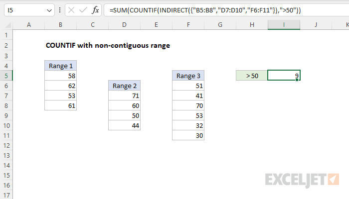
To count values in separate ranges with criteria, you can use the COUNTIF function together with INDIRECT and SUM. In the example shown, cell I5 contains this formula:
=SUM(COUNTIF(INDIRECT({"B5:B8","D7:D10","F6:F11"}),">50"))
The result is 9 since there are nine values greater than 50 in the three ranges shown.
Note: In Excel 365, the VSTACK and HSTACK functions offer a new approach to this problem. See below for an example.
Generic formula
=SUM(COUNTIF(INDIRECT({"rng1","rng2","rng3"}),criteria))
Explanation
In this example, the goal is to count values in three non-contiguous ranges with criteria. To be included in the count, values must be greater than 50. The COUNTIF counts the number of cells in a range that meet the given criteria. However, COUNTIF does not perform counts across different ranges. If you try to use COUNTIF with multiple ranges separated by commas, or in an array constant, you'll get an error. There are several ways to approach this problem, as explained below.
INDIRECT and COUNTIF
The INDIRECT function converts a given text string into a proper Excel reference:
=INDIRECT("A1") // returns A1
One approach is to provide the ranges as text in an array constant to INDIRECT like this:
INDIRECT({"B5:B8","D7:D10","F6:F11"})
Then pass the result from INDIRECT into the COUNTIF function like this:
=COUNTIF(INDIRECT({"B5:B8","D7:D10","F6:F11"}),">50")
INDIRECT will evaluate the text values and pass the references into COUNTIF as the range argument. For reasons mysterious, COUNTIF will accept the result from INDIRECT without complaint. Because COUNTIF receives more than one range, it will return more than one result in an array like this:
={4,2,3}
The three numbers in this array are the counts of numbers greater than 50 in each of the three ranges. To "catch" these results and return a total, we use the SUM function:
=SUM({4,2,3}) // returns 9
The SUM function then returns the sum of all values, 9. Although this is an array formula, it does not require CSE, since we are using an array constant.
Note: INDIRECT is a volatile function and can impact workbook performance.
More than one COUNTIF
Another way to solve this problem is to use more than one COUNTIF:
=COUNTIF(B5:B8,">50")+COUNTIF(D7:D10,">50")+COUNTIF(F6:F11,">50")
With a limited number of ranges, this approach may be easier to implement. It avoids possible performance impacts of INDIRECT and allows a normal formula syntax for ranges, so ranges will update automatically with worksheet changes. The INDIRECT example above relies on text strings that need to be updated manually.
VSTACK function
In current versions of Excel, a better approach is to first combine the ranges, and then perform the conditional count. To combine all three ranges vertically, you can use the VSTACK function:
=VSTACK(B5:B8,D7:D10,F6:F11)
The result from VSTACK is a single array with 14 values. Unfortunately, we can't pass this result into the COUNTIF function, because COUNTIF is in a group of functions that require actual ranges. However, we can use the SUM function and Boolean algebra to perform the conditional count. The complete formula looks like this:
=SUM(--(VSTACK(B5:B8,D7:D10,F6:F11)>50))
After VSTACK runs, and all values are checked with >50, we have an array of 14 TRUE and FALSE values like this:
{TRUE;TRUE;TRUE;TRUE;TRUE;TRUE;FALSE;FALSE;TRUE;FALSE;TRUE;TRUE;FALSE;FALSE}
The double negative (--) is used to convert the TRUE and FALSE values to 1s and 0s, and the resulting array is returned directly to the SUM function:
=SUM({1;1;1;1;1;1;0;0;1;0;1;1;0;0}) // returns 9
The SUM function sums the array and returns 9 as a final result.