Summary
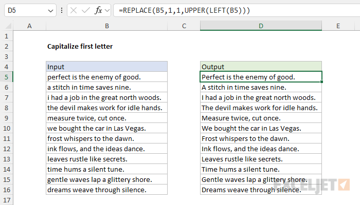
To capitalize the first letter in a text string, you can use a formula based on the REPLACE function, the UPPER function, and the LEFT function. In the example shown, the formula in D5 is:
=REPLACE(B5,1,1,UPPER(LEFT(B5)))
As the formula is copied down, it returns each sentence in column B with the first letter capitalized. All other letters in the sentence remain unchanged.
Generic formula
=REPLACE(A1,1,1,UPPER(LEFT(A1)))
Explanation
One of the most important skills to learn with Excel formulas is the concept of nesting. Put simply, nesting just means putting one function inside another. Nesting is super useful, but it does take some practice. You have to learn to read a formula from the inside out. The formulas below are good examples of nesting. Practice reading the formulas starting with the innermost functions.
In this example, the goal is to capitalize the first letter in a text string with a formula in Excel. This involves a bit of creative thinking because Excel does not offer a built-in function to capitalize only the first letter in a text string, unlike many other languages. This article explains a few approaches to the problem, including the formula featured in the worksheet above.
What about the PROPER function?
The simplest way to capitalize the first letter in a text string is to use the PROPER function, which is designed to capitalize words. For example, if we give PROPER the word "apple", PROPER returns "Apple":
=PROPER("apple") // returns "Apple"
This works very nicely for a single word or a person's name. However, it won't work in the worksheet shown because PROPER will capitalize all words. For example, If we give PROPER the text string "an apple a day", we get back "An Apple A Day":
=PROPER("an apple a day") // returns "An Apple A Day"
PROPER is a handy function, but not well suited to this problem. We need a different approach.
LEFT, UPPER, MID, and LEN
Another solution to this problem is to take a more literal approach: extract the first letter in the text string, capitalize it, and then concatenate the result to the remaining characters. This can be done with the formula below, which is based on four separate functions - LEFT, UPPER, MID, and LEN:
=UPPER(LEFT(B5))&MID(B5,2,LEN(B5)-1)
This is an example of nesting functions in Excel. Notice that the LEFT function is nested inside UPPER, and the LEN function is nested inside the MID function. The way to read nested functions is from the inside out:
- The LEFT function grabs the first letter.
- The UPPER function capitalizes the first letter.
- The LEN function calculates the length of the sentence.
- The MID function uses the length to get all remaining characters.
- The results from #2 and #4 are joined with concatenation.
The first expression uses the LEFT function to extract the first letter and the UPPER function to capitalize the first letter:
=UPPER(LEFT(B5))
Note that there is no need to enter 1 for num_chars in LEFT since it is an optional argument that defaults to 1.
Since cell B5 contains the text string "perfect is the enemy of good", this part of the formula evaluates like this:
=UPPER(LEFT(B5))
=UPPER(LEFT("perfect is the enemy of good"))
=UPPER("p")
="P"
The second expression extracts the remaining characters with the MID function:
MID(B5,2,LEN(B5)-1)
The text comes from B5, the start number is hardcoded as 2, and num_chars is provided by subtracting 1 from the result of the LEN function, which becomes 28:
=MID(B5,2,LEN(B5)-1)
=MID(B5,2,29-1))
=MID(B5,2,28))
="erfect is the enemy of good"
We subtract 1 because we have already dealt with the first character in the text string. However, MID won't complain if we ask for more characters than exist (it will simply extract everything), so technically we could omit the subtraction step and the formula will still return the same result.
Finally, the result from the first expression is joined to the result from the second expression with concatenation by using the ampersand (&) operator:
=UPPER(LEFT(B5))&MID(B5,2,LEN(B5)-1)
="P"&"erfect is the enemy of good"
="Perfect is the enemy of good"
This formula works fine for the problem as stated: it will capitalize the first letter of the sentence and leave all remaining characters unchanged. But do we need four functions to perform this task? Can't we do better?
Yes, we can. If we move to a formula based on the REPLACE function...
The REPLACE function
The REPLACE function is designed to replace one or more characters in a text string specified by location with another text string. For example, we can replace the last 3 letters in "ABCDEF" with "XYZ" like this:
=REPLACE("ABCDEF",4,3,"XYZ") // returns "ABCXYZ"
The arguments for REPLACE are provided as follows:
- old_text - "ABCDEF"
- start_num - 4
- num_chars - 3
- new_text - "XYZ"
In other words, REPLACE swaps three characters starting at character 4 with "XYZ". We can use the REPLACE function to solve this problem by replacing the first letter with a capitalized version of itself. This is the approach seen in the worksheet shown, where the formula in cell D5 is:
=REPLACE(B5,1,1,UPPER(LEFT(B5)))
Again, we have a great example of nesting. Notice that the LEFT function is nested inside the UPPER function which is itself nested inside the REPLACE function:
- The LEFT function grabs the first letter.
- The UPPER function capitalizes the first letter.
- The REPLACE function replaces the first letter with a capitalized version.
The formula evaluates like this:
=REPLACE(B5,1,1,UPPER(LEFT(B5)))
=REPLACE(B5,1,1,UPPER(LEFT("perfect is the enemy of good.")))
=REPLACE(B5,1,1,UPPER("p"))
=REPLACE(B5,1,1,"P")
="Perfect is the enemy of good."
Compared to the previous formula, this formula only needs three functions and doesn't require concatenation at all. The REPLACE does the work of replacing the first letter in place, leaving all remaining characters unaffected.
Note: If you do want to force all remaining characters to be lowercase, see the modification below.
Lowercase all the rest
If you want to lowercase everything but the first letter, just wrap the text given to REPLACE in the LOWER function like this
=REPLACE(LOWER(B5),1,1,UPPER(LEFT(B5)))
The formula will work the same as before. The only difference is that the REPLACE function will begin with an entirely lowercase text string.