Summary
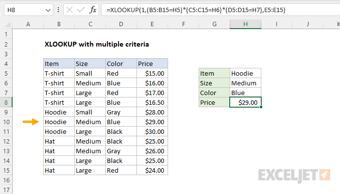
The best way to use XLOOKUP with multiple criteria is to use Boolean logic to apply conditions. In the example shown, the formula in H8 is:
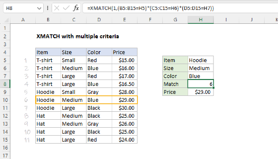
=XLOOKUP(1,(B5:B15=H5)*(C5:C15=H6)*(D5:D15=H7),E5:E15)
XLOOKUP returns $29.00, the price for a Medium Blue Hoodie. Note the lookup_value in XLOOKUP is 1 since the logical expressions in lookup_array create an array of 1s and 0s. Read below for details.
Note: in older versions of Excel, you can use the same approach with INDEX and MATCH.
Generic formula
=XLOOKUP(1,(criteria1)*(criteria2)*(criteria3),data)
Explanation
In this example, the goal is to look up a price using XLOOKUP with multiple criteria. To be more specific, we want to look up a price based on Item, Size, and Color. At a glance, this seems like a difficult problem because XLOOKUP only has one value for lookup_value and lookup_array. How can we configure XLOOKUP to consider values in multiple columns? The trick is to construct the lookup array we need using Boolean logic, then configure XLOOKUP to look for the number 1. This approach is explained below.
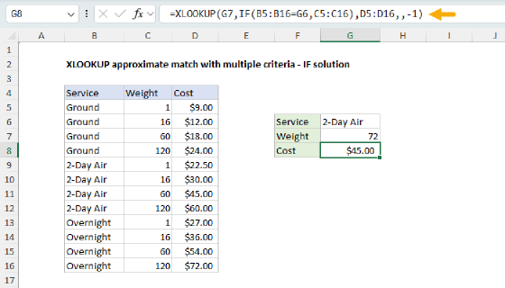
This examples "exact match" criteria. If you need an approximate match as a final result, see XLOOKUP approximate match with multiple criteria.
Basic XLOOKUP
The most basic use of XLOOKUP involves just three arguments:
=XLOOKUP(lookup_value,lookup_array,result_array)
Lookup_value is the value you are looking for, lookup_array is the range you are looking in, and result_array contains the value you want to return. There is no obvious way to supply multiple criteria.
Boolean Logic
This formula works around this limitation by using Boolean logic to create a temporary array of ones and zeros to represent rows matching all 3 criteria, then asking XLOOKUP to find the first 1 in the array. The temporary array of ones and zeros is generated with this snippet:
(B5:B15=H5)*(C5:C15=H6)*(D5:D15=H7)
Here we compare the item entered in H5 against all items, the size in H6 against all sizes, and the color in H7 against all colors. The initial result is three arrays of TRUE/FALSE values like this:
{FALSE;FALSE;FALSE;FALSE;TRUE;TRUE;TRUE;FALSE;FALSE;FALSE;FALSE}*{FALSE;TRUE;FALSE;FALSE;FALSE;TRUE;FALSE;TRUE;TRUE;FALSE;FALSE}*{FALSE;TRUE;FALSE;TRUE;FALSE;TRUE;FALSE;FALSE;FALSE;FALSE;FALSE}
Tip: use F9 to see these results. Just select an expression in the formula bar, and press F9.
The math operation (multiplication) automatically converts the TRUE FALSE values to 1s and 0s:
{0;0;0;0;1;1;1;0;0;0;0}*{0;1;0;0;0;1;0;1;1;0;0}*{0;1;0;1;0;1;0;0;0;0;0}
After multiplication is complete, we have a single array like this:
{0;0;0;0;0;1;0;0;0;0;0}
This is the array returned to XLOOKUP as the lookup_array. Notice, the sixth value in the array is 1. This corresponds to the sixth row in the data, which contains a Medium Blue Hoodie. Because our lookup_array contains only 1s and 0s, we set the lookup_value to 1. At this point, we can rewrite the formula like this:
=XLOOKUP(1,{0;0;0;0;0;1;0;0;0;0;0},E5:E15) // returns 29
XLOOKUP locates the 1 in the sixth row of the lookup_array and returns the sixth value in the return_array (E5:E15). This is $29.00, the price of a Medium Blue Hoodie.
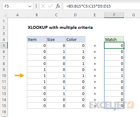
Array visualization
The arrays explained above can be difficult to visualize. The image below shows the process. Columns B, C, and D correspond to the data in the example, after being compared to the values in H5, H6, and H7. Column F is created by multiplying the three columns together. This is the array delivered to XLOOKUP as the lookup_array.
Alternative with concatenation
In simple cases like this example, you will sometimes see an alternative approach that uses concatenation instead of Boolean logic. The formula looks like this:
=XLOOKUP(H5&H6&H7,B5:B15&C5:C15&D5:D15,E5:E15)
The lookup_value is created by joining H5, H6, and H7 using concatenation:
=XLOOKUP(H5&H6&H7
This results in the string "HoodieMediumBlue". The lookup_array is created in a similar way, except we are now joining ranges:
=XLOOKUP(H5&H6&H7,B5:B15&C5:C15&D5:D15
The return_array is supplied as a normal range, E5:E15:
=XLOOKUP(H5&H6&H7,B5:B15&C5:C15&D5:D15,E5:E15)
In essence, we are gluing together the values we need for criteria in the lookup_array, then looking for a value we created by joining together the Item, Size, and Color that we want to find. In this configuration, XLOOKUP returns $29.00 as before.
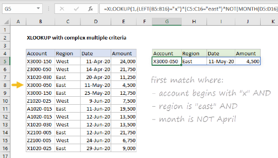
This approach works in simple scenarios, but the Boolean Logic approach is far more flexible and powerful, so I recommend you use that method instead of concatenation. For an example of a problem that cannot be solved with concatenation, see XLOOKUP with complex multiple criteria.
INDEX and MATCH
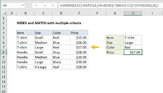
XLOOKUP is only available in newer versions of Excel, but you can use the same technique with INDEX and MATCH, which will work in any version. The formula below uses INDEX and MATCH with Boolean logic to achieve the same result:
=INDEX(E5:E15,MATCH(1,(B5:B15=H5)*(C5:C15=H6)*(D5:D15=H7),0))
Note: in Legacy Excel, this is an array formula and needs to be entered with Control + Shift + Enter. In newer versions of Excel that support dynamic array formulas, this formula will work seamlessly.
For more details and a sample workbook, see INDEX and MATCH with multiple criteria.