Summary
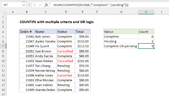
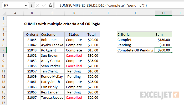
To sum based on multiple criteria using OR logic, you can use the SUMIFS function with an array constant. In the example shown, the formula in H7 is:
=SUM(SUMIFS(E5:E16,D5:D16,{"complete","pending"}))
The result is $200, the total of all orders with a status of "Complete" or "Pending". Note that the SUMIFS function is not case-sensitive.
Generic formula
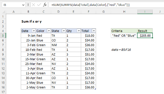
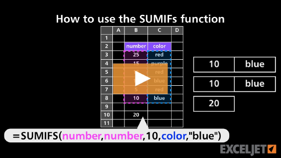
=SUM(SUMIFS(sum_range,criteria_range,{"red","blue"}))
Explanation
In this example, the goal is to sum the value of orders that have a status of "Complete" or "Pending". This is a slightly tricky problem in Excel because the SUMIFS function is designed for conditional sums based on multiple criteria, but all criteria must be TRUE in order for a value to be included in the sum. In other words, the criteria used in the SUMIFS function are joined with AND logic, not OR logic. In simple scenarios, an easy solution is to use the SUMIFS function with an array constant.
SUMIFS function
The SUMIFS function sums the values in a range that meet multiple criteria. It is similar to the SUMIF function, which only allows a single condition, but SUMIFS allows multiple criteria, using AND logic. This can be illustrated with the following formulas:
=SUMIFS(E5:E16,D5:D16,"complete") // returns 150
=SUMIFS(E5:E16,D5:D16,"pending") // returns 50
=SUMIFS(E5:E16,D5:D16,"complete",D5:D16,"pending") // returns 0
Notice the first two formulas correctly return the total of complete and pending orders, but the last formula returns zero because an order cannot be "Complete" and "Pending" at the same time. This is because the SUMIFS function only allows AND logic – all conditions must be TRUE for a value to be included in the sum.
SUMIFS + SUMIFS
One straightforward solution is to use SUMIFS twice in a formula like this:
=SUMIFS(E5:E16,D5:D16,"complete")+SUMIFS(E5:E16,D5:D16,"pending")
This formula returns a correct result of $200, but it is redundant and doesn't scale well.
SUMIFS + array constant
Another option is to supply SUMIFS with an array constant that holds more than one condition, like this:
=SUMIFS(E5:E16,D5:D16,{"complete","pending"}) // returns {150,50}
Through a formula behavior called "lifting", this will cause SUMIFS to be evaluated twice, once for "complete" and once for "pending", and SUMIFS will return two results in an array like this:
{150,50}
If you enter the formula above in the latest version of Excel, which supports dynamic array formulas, you will see both results spill into a range that contains two cells. Because we want a single result, we nest the SUMIFS function in the SUM function like this:
=SUM(SUMIFS(E5:E16,D5:D16,{"complete","pending"}))
This is the formula used in the worksheet shown. The formula evaluates like this:
=SUM(SUMIFS(E5:E16,D5:D16,{"complete","pending"}))
=SUM({150,50})
=200
The SUMIFS function returns two results in an array: 250 and 50. This array is returned to the SUM function, which returns a final result of 200.
With wildcards
You can use wildcards in the criteria if needed. For example, to sum items that contain "red" or "blue" anywhere in the criteria_range, you can use:
=SUM(SUMIFS(sum_range,criteria_range,{"*red*","*blue*"}))
Adding more conditions
You can add more conditions to this formula, but you'll need to use a horizontal array for one set of criteria and a vertical array for the other. So, for example, to sum orders that are "Complete" or "Pending", when the customer is "Andy Garcia" or "Bob Jones", you can use a formula like this:
=SUM(SUMIFS(E4:E16,D4:D16,{"complete","pending"},C4:C16,{"Bob Jones";"Andy Garcia"}))
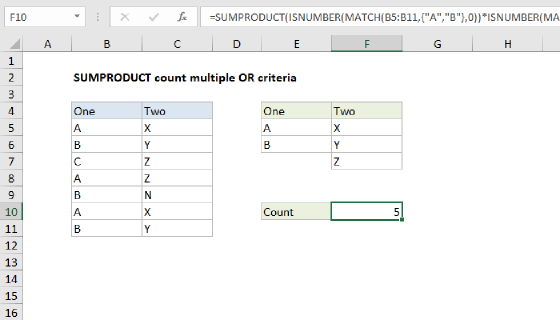
Note the semicolons in the second array constant represent a vertical array. This works because Excel "pairs" elements in the two array constants and returns a two-dimensional array of results. To apply additional criteria, you will want to move to a formula based on SUMPRODUCT.
Cell references for criteria
You can't use cell references inside an array constant; you must use a proper range. When you switch from array constants to ranges, the formula becomes an array formula in older versions of Excel and must be entered with control + shift + enter:
={SUM(SUMIFS(range1,range2,range3))}
Where range1 is the sum range, range2 is the criteria range, and range3 contains multiple criteria on the worksheet. With two OR criteria, you'll need to use horizontal and vertical arrays as explained above.
Note: this formula will work fine in modern versions of Excel that support dynamic array formulas without special handling. In Exceln 2019 or older, you will need to enter the formula as an array formula with Ctrl + Shift + Enter.