The term "lifting" (also called "auto-lifting") refers to an array behavior that occurs in Excel formulas. Lifting is an automatic, element-wise evaluation of an operation or function over an array. When an operator or function that typically accepts scalar (single) values is given one or more arrays, Excel “lifts” the operation so it is applied to each element and returns an array of results. If this array is the final result of a formula, the array spills into the worksheet according to the dimensions of the array. In the case of a function, when you give a range or array to a function not programmed to accept arrays natively, Excel will "lift" the function and call it multiple times, one time for each value in the array. The result is an array with the same dimensions as the input array that spills onto the worksheet.
Example
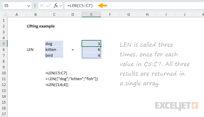
The example shown illustrates what happens if you call the LEN function on the range C5:C7, which contains three values. LEN returns the count of characters in a text string. LEN isn't programmed to handle arrays natively, so when given the range C5:C5, LEN is called three times, once for each value in the range. Because the incoming range contains three cells, the result from LEN is an array that contains three counts. For the worksheet shown above, this is how the formula evaluates:
=LEN(C5:C7)
=LEN({"dog";"kitten";"fish"})
={3;6;4}
Because the formula is entered in cell E5, the results spill into E5:E7. Notice the result is a vertical array with three values, just like the source range.
In Excel 2021 and later, which supports dynamic array formulas, you will see lifting happen in real-time as multiple results spill onto the worksheet. In earlier versions of Excel, lifting still occurs, but only one result is displayed in the cell that contains the formula.
Flavors of lifting
Several different scenarios involve lifting in Excel. If a scalar is combined with an array, the scalar is lifted across the array (often called scalar lifting); if two arrays of the same shape are combined, Excel evaluates them pairwise; and if shapes differ, Excel first broadcasts to a compatible shape, then lifts the operation.
- Scalar lifting - A scalar (single value or scalar function) is applied across each element in an array.
=A5:A10 + 1adds 1 to each value in A1:A10. Cell A1 holds the formula; the results spill.=LEN(A1:A10)returns an array of text lengths for each cell in A1:A10.
- Pairwise lifting - Two arrays of the same shape are combined element by element.
=B5:B10 * C5:C10multiplies each pair of corresponding values.
- Broadcast + lifting - When array shapes differ, Excel "broadcasts" the smaller array to match the larger one, then applies the operation element-wise
B1:B10 * D1broadcasts D1 down to ten rows to match B1:B10 before multiplication.
Some Excel functions, like EOMONTH, resist lifting and spilling when provided a range — they won't automatically spill results without extra help. For more details and a list of functions that have this problem, see: Why some functions won't spill.
Dealing with multiple results
When lifting occurs in a formula, there will be multiple results that spill onto the worksheet. However, you can also modify your formula to process the results and return a single value. In the example shown, LEN returns three separate counts in an array. If we wanted to output a single count to indicate the total characters in the range, we could wrap LEN in the SUM function like this:
=SUM(LEN(C5:C7)) // returns 13
The final result will be 13, the sum of 3 + 6 + 4.
Note: In an older version of Excel, use the SUMPRODUCT function instead of the SUM function.


