Summary
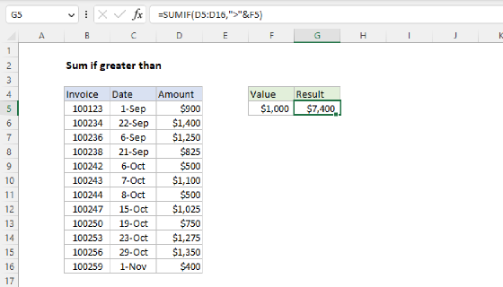
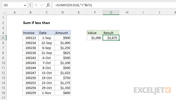
To sum values less than a given value, you can use the SUMIF function or the SUMIFS function. In the example shown, cell G5 contains this formula:
=SUMIF(D5:D16,"<"&F5)
With $1,000 in cell F5, this formula returns $3,875, the sum of values in D5:D16 less than $1,000.
Generic formula
=SUMIF(D5:D16,"<"&A1)
Explanation
In this example, the goal is to sum values in the range D5:D16 when they are less than the value entered in cell F5. This problem can be easily solved with the SUMIF function or the SUMIFS function. The main challenge in this problem is the syntax needed for cell F5 in the criteria, which involves concatenation.
SUMIF function
The SUMIF function is designed to sum cells based on a single condition. The generic syntax for SUMIF looks like this:
=SUMIF(range,criteria,sum_range)
For example, to sum values in D5:D16 that are less than $1,000, we can use the SUMIF function like this:
=SUMIF(D5:D16,"<1000") // returns 3875
We don't need to enter a sum_range, because D5:D16 contains both the values we want to test and the values we want to sum. When this formula is entered on the worksheet shown, it returns $3,875, the sum of values in D5:D16 that are less than $1,000.
Hardcoded value versus cell reference
The formula above is an example of hardcoding a value into a formula, which is generally a bad practice, because it makes the formula less transparent and harder to maintain. A better approach is to expose the value on the worksheet where it can be easily changed, as seen in the worksheet shown. This is the tricky part of the formula because we need to use concatenation to join the operator ("<") to the cell reference F5. The updated formula looks like this:
=SUMIF(D5:D16,"<"&F5)
Notice the operator is in double quotes (">") and joined to cell F5 with an ampersand (&). When Excel evaluates this formula, it will start with the criteria, first retrieving the value from cell F5, then joining the value to the operator. After evaluating criteria, the formula will look like this:
=SUMIF(D5:D16,"<1000")
Notice this is exactly the same formula we started with above. However, by using a reference to F5 the threshold value can easily be changed at any time. For more information about SUMIF, see this page. For more on concatenation, see this page.
SUMIFS function
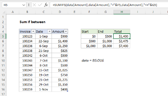
This formula can also be solved with the SUMIFS function, which is designed to sum cells in a range with multiple criteria. The syntax for SUMIFS is similar, but the order of the arguments is different. With a single condition, the generic syntax for SUMIFS looks like this:
=SUMIFS(sum_range,range1,criteria1) // 1 condition
Unlike the SUMIF function, the sum_range argument comes first and not last, and is not optional. In general, this is more logical, but it does make the formula a little longer when working with just one condition. The equivalent SUMIFS formula looks like this:
=SUMIFS(D5:D16,D5:D16,"<"&F5)
Notice the criteria in this formula is exactly the same as what we used in SUMIFS above. However, we need to enter the range D5:D16 two times: once as sum_range, and once for range. When we enter this formula it returns $3,875, the sum of all values less than $1,000 in the range D5:D16. For information about SUMIFS, see this page.