Summary
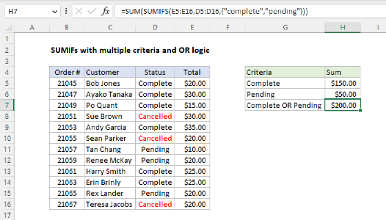
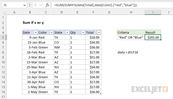
To sum numbers when corresponding cells are equal to x or y, you can use the SUMIFS function with the SUM function and an array constant. In the example shown, the formula in cell I5 is:
=SUM(SUMIFS(data[Total],data[Color],{"red","blue"}))
Where data is an Excel Table in the range B5:F16. The result is $205, the sum of Total where the Color is "Red" OR "Blue". Note the SUMIFS function is not case-sensitive.
Generic formula
=SUM(SUMIFS(range1,range2,{"red","blue"}))
Explanation
In this example, the goal is to sum Total when the corresponding Color is either "Red" or "Blue". For convenience, all data is in an Excel Table named data. This is a tricky problem, because the solution is not obvious. The go-to function for conditional sums is the SUMIFS function. However, when using SUMIFS with multiple criteria, all conditions must be TRUE. This means that multiple conditions are joined with AND logic and there is no direct way to apply conditions with OR logic. One solution is to use an array constant with SUMIFS, then sum the results with the SUM function. Another option is to use SUMIFS twice.
SUMIFS + SUMIFS
Before looking at the more advanced option shown in the example, it's important to note that we can solve this problem with two calls to SUMIFS like this:
=SUMIFS(data[Total],data[Color],"red")+
SUMIFS(data[Total],data[Color],"blue")
The first SUMIFS sums Total where the color is "Red", and the second SUMIFS sums Total where the color is "Blue". By adding the two functions together in one formula, we effectively get a sum of Total where the color is either "Red" or "Blue".
SUMIFS + array constant
A more elegant solution is to give the SUMIFS function more than one value for the criteria, in an array constant. To do this, construct a normal SUMIFS formula, but supply criteria in array syntax like this:
{"red","blue"} // array constant
Placing the array constant inside SUMIFS as criteria1, we have:
SUMIFS(data[Total],data[Color],{"red","blue"})
In this configuration, SUMIFS will return two sums: one for totals where the color is "Red" and one for totals where the color is "Blue". These results will be returned in an array like this:
{86,119} // result from SUMIFS
In the latest version of Excel you will see these results spill onto the worksheet into two cells. However, we don't want two results on the worksheet (we want a single result) so we wrap the SUMIFS function inside the SUM function like this:
=SUM(SUMIFS(data[Total],data[Color],{"red","blue"}))
Now SUMIFS will return the array to SUM:
=SUM({86,119}) // returns 205
and the SUM function will return the final result, 205.
Criteria as reference
You can also supply criteria as a cell reference instead of an array constant. For example, with "Red" in cell A1 and "Blue" in cell A2, you can use a formula like this:
=SUM(SUMIFS(data[Total],data[Color],A1:A2))
In the latest version of Excel, this formula will work as-is, with no special handling. In Legacy Excel, you will need to enter as an array formula with control + shift + enter.
SUMPRODUCT alternative
You can also use the SUMPRODUCT function to sum cells with OR logic with a formula like this
=SUMPRODUCT(--ISNUMBER(MATCH(data[Color],{"red","blue"},0))*data[Total])
This formula uses the MATCH function and the ISNUMBER function to create a Boolean array that is then multiplied by data[Total] to get a final result. This is a flexible approach that works nicely in situations where SUMIFS can't be used.
Note: in the current version of Excel you can use the SUM function instead of SUMPRODUCT. See Why SUMPRODUCT?