Summary
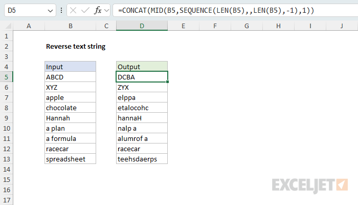
To reverse a text string, you can use a formula based on the MID, SEQUENCE, and CONCAT functions. In the example shown, the formula in D5, copied down, is:
=CONCAT(MID(B5,SEQUENCE(LEN(B5),,LEN(B5),-1),1))
MID extracts the characters in reverse order, and CONCAT joins them back together, so "ABCD" becomes "DCBA". SEQUENCE is available in Excel 2021+ and Excel 365. For Excel 2019, see the formula below.
Generic formula
=CONCAT(MID(A1,SEQUENCE(LEN(A1),,LEN(A1),-1),1))
Explanation
In this example, the goal is to reverse the text in column B, so that the last character comes first. For example, "ABCD" in B5 should become "DCBA" in D5. Excel has no function that reverses text, but you can split the text into characters in reverse order, then join the characters back together.
Extract characters in reverse order
At the core, this formula uses the MID function to extract each character of a text string in reverse order. MID normally extracts characters from one starting position. But if you give MID an array of starting positions, it returns one result for each, and the trick is to supply the positions in descending order. We can do this with the SEQUENCE function and the LEN function like so:
SEQUENCE(LEN(B5),,LEN(B5),-1)
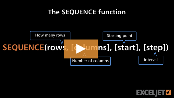
Inside SEQUENCE, LEN returns the count of characters in B5, 4. This result is used both for the rows argument and the start argument. To count in descending order, -1 is provided for the step argument:
SEQUENCE(4,,4,-1) // returns {4;3;2;1}
This array is delivered to the MID function as the start_num argument, with 1 for num_chars:
MID(B5,{4;3;2;1},1) // returns {"D";"C";"B";"A"}
Because LEN counts the characters in each cell, the formula adjusts to text of any length: "spreadsheet" in B13 has 11 characters, and SEQUENCE returns 11 positions.
Join the characters
The array from MID is returned to the CONCAT function, which joins the characters together and returns the final result, "DCBA":
=CONCAT({"D";"C";"B";"A"}) // returns "DCBA"
The TEXTJOIN function also works, with an empty string ("") as the delimiter: =TEXTJOIN("",TRUE,MID(B5,SEQUENCE(LEN(B5),,LEN(B5),-1),1)).
With either approach above, CONCAT and TEXTJOIN always return text, so a number like 12345 becomes the text "54321".
Empty cells
If B5 is empty, LEN returns zero, and SEQUENCE can't create an array with zero rows, so the formula returns a #CALC! error. To trap this error and return an empty string instead, test for an empty cell first with the IF function like this:
=IF(B5="","",CONCAT(MID(B5,SEQUENCE(LEN(B5),,LEN(B5),-1),1)))
Excel 2019
Excel 2019 has TEXTJOIN but not SEQUENCE. To create the positions, use the ROW and INDIRECT functions instead:
=TEXTJOIN("",TRUE,MID(B5,LEN(B5)-ROW(INDIRECT("1:"&LEN(B5)))+1,1))
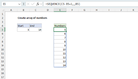
With "ABCD" in B5, ROW(INDIRECT("1:4")) returns {1;2;3;4}, and subtracting these numbers from LEN(B5)+1 reverses them to {4;3;2;1}. In Excel 2019, this is an array formula and must be entered with Control + Shift + Enter. An empty cell returns #REF!, because "1:0" is not a valid reference. For more about this technique, see Create array of numbers.