Summary
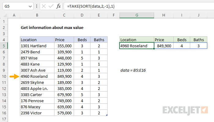
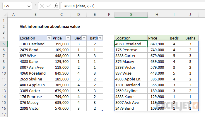
To get information related to the maximum value in a range, you can use a formula based on the TAKE function and the SORT function. In the example shown, the formula in G5 is:
=TAKE(SORT(data,2,-1),1)
where data is an Excel Table in the range B5:E16. The result is all information related to the property at 4960 Roseland, which has the maximum price in the data shown.
Note: In older versions of Excel without TAKE and SORT, you can use an INDEX and MATCH formula. See below for details.
Generic formula
=TAKE(SORT(range,2,-1),1)
Explanation
An interesting problem in Excel is how to look up information related to the maximum value in a set of data. For example, if you have a dataset of property listings and prices, you might want to find details about the property with the highest price. The best way to solve this problem depends on which version of Excel you use. In Excel 2019 and earlier, the classic solution is to use the MAX function to find the maximum value, then use this value in an INDEX and MATCH formula as the lookup value. In the current version of Excel, there is a better way. Instead of performing a lookup operation, you can use the SORT function to sort by price in descending order, and then use the TAKE function to retrieve the first row.
This new approach is simple and elegant, and it greatly simplifies many complicated formulas. The article explains the new approach based on SORT and TAKE, as well as the traditional approach based on INDEX and MATCH. Don’t forget to download the worksheet and try it out yourself.
The goal
The goal is to retrieve information related to the maximum price in the worksheet shown. Specifically, we want to return all four columns of data (Location, Price, Beds, and Baths) for the property with the highest price. If the data changes, the formula should automatically recalculate and display updated information. For convenience, all property information is in an Excel Table named data.
TAKE function
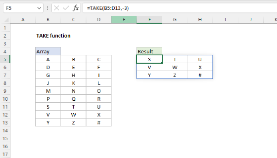
The TAKE function in Excel allows you to return a subset of a given array. The size of the array returned is determined by separate rows and columns arguments. The generic syntax looks like this:
=TAKE(range,rows,columns)
For example, to retrieve the first row in a range, you can use TAKE like this:
=TAKE(range,1) // get first row
When positive numbers are provided for rows or columns, TAKE will get values from the start of the array. When negative numbers are provided, TAKE will get values from the end of the array.
For more details, see How to use the TAKE function
SORT function
The SORT function in Excel allows you to sort a range or array in either ascending or descending order. For this problem, the generic syntax for SORT looks like this:
=SORT(array,sort_index,sort_order)
Sort_index is a number representing the column to sort by. Sort_order controls sort direction and can be provided as 1 (ascending) or -1 (descending). For example, to sort a range by the second column of data, you can use SORT like this:
=SORT(range,2,1) // sort by column 2 ascending
=SORT(range,2,-1) // sort by column 2 descending
For more details, see How to use the SORT function
TAKE with SORT
An efficient way to solve this problem is to combine the TAKE and SORT functions. In the example shown, we want to get all information related to the most expensive property. This can be done with a formula that combines SORT and TAKE like this:
=TAKE(SORT(data,2,-1),1)
Working from the inside out, the SORT function first sorts the data by price in descending order:
SORT(data,2,-1) // sort descending by price
By itself, SORT returns all data in a single array, with the most expensive property listed first:
The sorted array is then handed off to the TAKE function, which is configured to return just row 1:
=TAKE(SORT(data,2,-1),1)
The result from TAKE is an array with 4 values like this:
{"4960 Roseland",849900,4,3}
This array lands in cell G5, and the 4 values spill into the range G5:J5.
FILTER with LARGE
Because this is Excel, there is always another way to solve the same problem :) Here is another good formula:
=FILTER(data,data[Price]=LARGE(data[Price],1))
In this formula, we use the LARGE function to get the maximum price, then use the FILTER function to extract rows where the price equals the maximum price. For more details, see How to use the FILTER function and How to use the LARGE function.
INDEX and MATCH
If you are using an older version of Excel without TAKE, SORT, or FILTER, you can solve this problem with an alternative method based on an INDEX and MATCH formula like this:
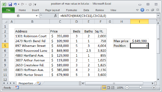
=INDEX(data,MATCH(MAX(data[Price]),data[Price],0),1)
Working from the inside out, the MAX function first extracts the maximum value from the Price column:
MAX(data[Price]) // returns 849900
This value is then provided to the MATCH function as the lookup_value, with lookup_array given as the Price column, and match_type is set to zero (0) for an exact match:
MATCH(849900,data[Price],0) // returns 6
Using this information, the MATCH function returns the row number of the maximum price (6) directly to INDEX as row_num:
=INDEX(data,6,1) // returns "4960 Roseland"
The INDEX function then returns the value at row 6 and column 1 of the table, which is "4960 Roseland". In case of duplicates (i.e., two or more max values that are the same), the formula will return info for the first match, the default behavior of the MATCH function. The other three columns can be retrieved in the same way by adjusting the column number as needed:
=INDEX(data,MATCH(MAX(data[Price]),data[Price],0),2) // price
=INDEX(data,MATCH(MAX(data[Price]),data[Price],0),3) // beds
=INDEX(data,MATCH(MAX(data[Price]),data[Price],0),4) // baths
For a complete overview of INDEX with MATCH, see How to use INDEX and MATCH.