Explanation
The LARGE function is an easy way to get the nth largest value in a range:
 =LARGE(range,1) // 1st largest
 =LARGE(range,2) // 2nd largest
 =LARGE(range,3) // 3rd largest
In this example, we can use the LARGE function to get a highest score, then use the score like a "key" to retrieve the associated name with INDEX and MATCH. Notice we are picking up the values for n from the range F5:F7, in order to get the 1st, 2nd, and 3rd highest scores.
The twist however in this case is that we need to distinguish between scores in group A and group B. In other words, we need to apply criteria. We do this with the IF function, which is used to "filter" values before they are evaluated with LARGE. As a generic example, to get the largest value (i.e. 1st value) in range2 where range 1 = "A", you can use a formula like this:
LARGE(IF(range="A",range2),1)
Note: using IF this way makes this an array formula.
Working from the inside out, the first step is to get the "1st" largest value in the data associated with Group A with the LARGE function:
LARGE(IF(group="A",score),F5)
In this case, the value in F5 is 1, so we are asking for the top score in Group A. When the IF function is evaluated, it tests each value in the named range group. The named range score is provided for value_if_true. This generates a new array, which is returned directly to the LARGE function:
LARGE({79;FALSE;93;FALSE;83;FALSE;67;FALSE;85;FALSE;69;FALSE},1)
Notice the only scores that survive the filter are from Group A. LARGE then returns the highest remaining score, 93, directly to the MATCH function as a lookup value. We can now simplify the formula to:
=INDEX(name,MATCH(93,IF(group="A",score),0))
Now we can see that the MATCH function is configured to use the same filtered array we saw above. The IF function again filters out unwanted values, and the MATCH portion of the formula resolves to:
MATCH(93,{79;FALSE;93;FALSE;83;FALSE;67;FALSE;85;FALSE;69;FALSE},0)
Since 93 appears in the 3rd position, MATCH returns 3 directly to the INDEX function:
=INDEX(name,3) // Hannah
Finally, the INDEX function returns the name in the 3rd row, "Hannah".
With XLOOKUP
The XLOOKUP function can also be used to solve this problem, using the same approach explained above:
=XLOOKUP(LARGE(IF(group="A",score),F5),IF(group="A",score),name)
As above, LARGE is configured to work with an array filtered by IF, and returns a result of 93 to XLOOKUP as the lookup value:
=XLOOKUP(93,IF(group="A",score),name) // Hannah
The lookup array is also created by using IF as a filter on scores from Group A. With the return array provided as name (B5:B16). XLOOKUP returns "Hannah" as the final result.
Notes
- To get the name of nth value with criteria, (i.e. limit results to group A or B) you will need to extend the formula to use additional logic.
- In Excel 365, the FILTER function is a better way to list top or bottom results dynamically. This approach will automatically handle ties.


