Summary
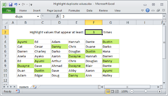
Excel contains a built-in preset for highlighting duplicate values with conditional formatting, but it only works at the cell level. If you want to highlight entire rows that are duplicates you'll need to use your own formula, as explained below.
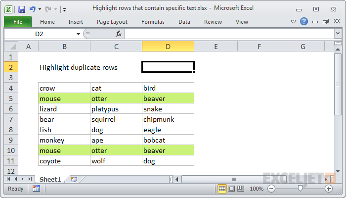
If you want to highlight duplicate rows in an unsorted set of data, and you don't want to add a helper column, you can use a formula that uses the COUNTIFS function to count duplicated values in each column of the data.
For example, if you have values in the cells B4:D11, and want to highlight entire duplicate rows, you can use rather ugly formula:
=COUNTIFS($B$4:$B$11,$B4,$C$4:$C$11,$C4,$D$4:$D$11,$D4)>1
Named ranges for a cleaner syntax
The reason the above formula is so ugly is that we need to fully lock each column range, then used a mixed reference to test each cell in each column. If you create named ranges for each column in the data: col_a, col_b, and col_c, the formula can be written with a much cleaner syntax:
=COUNTIFS(col_b,$B4,col_c,$C4,col_d,$D4)>1
Generic formula
=COUNTIFS(A:A,$A1,B:B,$B1,C:C,$C1)
Explanation
In the formula, COUNTIFS counts the number of times each value in a cell appears in its "parent" column. By definition, each value must appear at least once, so when the count > 1, the value must be a duplicate. The references are carefully locked so the formula will return true only when all 3 cells in a row appear more than once in their respective columns.
The helper column option "cheats" by combining all values in a row together in single cell using concatenation. Then COUNTIF simply counts the number of times this concatenated value appears in column D.
Helper column + concatenation
If you don't mind adding a helper column to your data, you can simplify the conditional formatting formula quite a bit. In a helper column, concatenate values from all columns. For example, add a formula in column E that looks like this:
=B4&C4&D4
Then use the following formula in the conditional formatting rule:
=COUNTIF($E$4:$E$11,$E4)>1
This is a much simpler rule, and you can hide the helper column if you like.
If you have a really large number of columns, you can use the TEXTJOIN function (Excel 2016 365) to perform concatenation using a range:
=TEXTJOIN(",",TRUE,A1:Z1)
You can then use COUNTIF as above.
SUMPRODUCT
If you're using a version of Excel before 2007, you can use SUMPRODUCT like this:
=SUMPRODUCT((col_b=$B4)*(col_c=$C4)*(col_d=$D4))>1