Summary
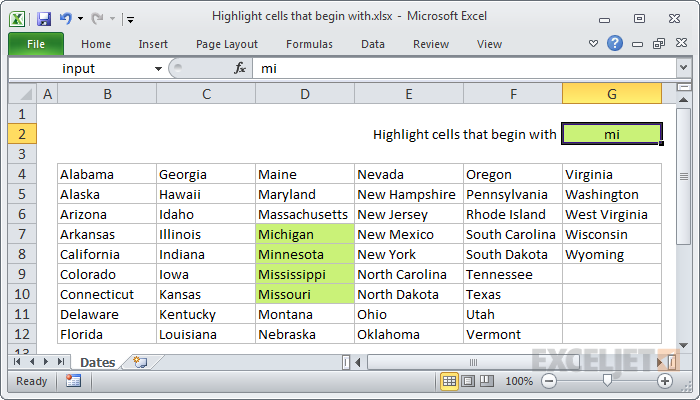
To highlight cells that begin with certain text, you can use a formula based on the SEARCH function to trigger a conditional formatting rule. In the example shown, the formula used to highlight values that begin with "mi" is:
=SEARCH($G$2,B4)=1
Here, G2 contains the text to search for, and B4 is the cell being evaluated. When this formula returns TRUE, it triggers a conditional formatting rule that applies a bright fill color to cells that begin with "mi", as seen in the worksheet above. The value in cell G2 can be changed at any time.
Note: Excel contains many built-in "presets" for highlighting values with conditional formatting, including a preset to highlight cells that begin with specific text. However, defining a rule based on your own formula provides more flexibility and power. For example, you can easily adapt the formula to perform a case-sensitive match, as explained below.
Generic formula
=SEARCH("substring",A1)=1
Explanation
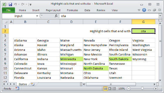
In this example, the goal is to apply conditional formatting to cells that begin with specific text, which is entered in cell G2. The highlighting is done automatically with a conditional formatting rule applied to the range B4:G12. The rule type is "Use a formula to determine which cells to format". The formula looks like this:
=SEARCH($G$2,B4)=1
G2 contains the text to search for, and B4 is the cell being tested. The formula is evaluated relative to the active cell at the time the rule is created for each cell in the range, which is B4. Each cell in B4:G12 is evaluated separately. Since B4 is entered as a relative reference, it will change to the cell being evaluated. Since cell G2 is entered as an absolute reference ($G$2), it will not change.
The formula uses the SEARCH function to match cells that begin with "mi". SEARCH returns a number that indicates a position when the text is found, and a #VALUE! error if the text is not found. When SEARCH returns the number 1, we know that the cell value begins with "mi" because the location of the text is 1. The formula returns TRUE when the position is 1 and FALSE for any other value. For example, in cell B4, the formula evaluates like this:
When this formula returns TRUE, it triggers a conditional formatting rule that applies a bright fill color to cells that begin with "mi", as seen in the worksheet above. The value in cell G2 can be changed at any time and the conditional formatting will instantly update.
With a named input cell
You can simplify the formula a bit by using a named range for cell G2. For example, if we name G2 "input" the formula can be revised as follows:
=SEARCH(input,B4)=1
The named range automatically behaves like an absolute reference so there is no need to lock any references.
Case-sensitive option
The SEARCH is not case-sensitive so the text "MI" and "mi" will be evaluated in the same way. If you need a case-sensitive version of the formula, you can use a formula based on the FIND function instead:
=FIND(input,B4)=1
Like the SEARCH function, FIND returns the position of the text as a number. However, FIND is automatically case-sensitive.