Summary
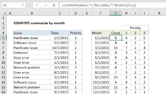
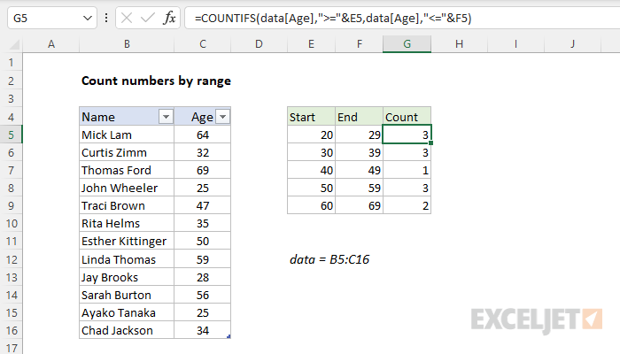
To count numeric data in specific ranges or brackets, you can use the COUNTIFS function. In the example shown, the formula in G5, copied down, is:
=COUNTIFS(data[Age],">="&E5,data[Age],"<="&F5)
where data is an Excel Table in the range B5:C16. As the formula is copied down, it returns a new count in each row using the Start and End values in columns E and F to determine a count.
Generic formula
=COUNTIFS(range,">=low",range,"<=high")
Explanation
In this example, the goal is to count ages in column C according to the brackets defined in columns E and F. All data is in an Excel Table named data defined in the range B5:C16. A simple way to solve this problem is with the COUNTIFS function. If you are using Excel 365 or Excel 2021, another easy way to solve this problem is with the FREQUENCY function. Both approaches are explained below.
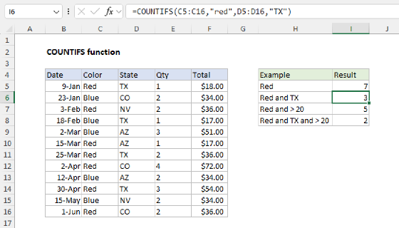
COUNTIFS function
The COUNTIFS function returns the count of cells that meet one or more criteria, and supports logical operators (>,<,<>,=) and wildcards (*,?) for partial matching. Conditions are supplied to COUNTIFS in the form of range/criteria pairs — each pair contains one range and the associated criteria for that range:
=COUNTIFS(range1,criteria1,range2,criteria2,etc)
Using this pattern we can count ages in brackets like this:
=COUNTIFS(data[Age],">=20",data[Age],"<=29") // 20-29
=COUNTIFS(data[Age],">=30",data[Age],"<=39") // 30-39
=COUNTIFS(data[Age],">=40",data[Age],"<=49") // 40-49
We are using the structured reference data[Age] for both ranges, since data is an Excel Table. Using an Excel Table means the table will expand automatically as new rows are added, and the counts will remain up to date.
Notice in the formulas above, we are hardcoding the numbers into the formula. This is generally considered a bad practice, since it's easy to make a mistake when entering the formula and it's more difficult to adjust the ranges later if needed, especially since each age bracket has its own unique formula. A better approach is to use ages already on the worksheet in columns E and F.
To do this, we need to concatenate the ages in columns E and F to the logical operators >= and <=. The final formula in G5 looks like this:
=COUNTIFS(data[Age],">="&E5,data[Age],"<="&F5)
Notice the operators are enclosed in double quotes ("") and attached to cell references E5 and F5 with an ampersand character (&). For a detailed overview of concatenation, see How to concatenate in Excel. As this formula is copied down, the reference to data[Age] behaves like an absolute reference and does not change, which means we can use the same formula for all five age brackets.
If you need a final bracket that captures all ages above 70, you can use a single condition like this:
=COUNTIFS(data[Age],">=70") // 70+
This formula will return a count of all ages greater than or equal to 70.
FREQUENCY function
If you are using Excel 365 or Excel 2021, where array formulas are native, a nice way to solve this problem is with the FREQUENCY function. The FREQUENCY function returns more than one value at a time and needs to be entered as a multi-cell array formula in Legacy Excel. In modern Excel, you can simply use a formula like this in cell G5:
FREQUENCY(data[Age],F5:F9)
Here, the data_array is given as data[Age] and the bins_array is given as F5:F9, the "End" values in column F. The FREQUENCY function performs the calculation and returns an array like this:
{3;3;1;3;2;0}
Each number represents a count, and the results automatically spill into multiple cells. Notice that by design, the FREQUENCY function always returns a count for one more bin than is provided. This is called the overflow bin, and represents the count of any values greater than the largest value in the bins_array. To suppress this last count, you can nest the FREQUENCY function inside the DROP function like this:
=DROP(FREQUENCY(data[Age],F5:F9),-1)
The DROP function will remove the last row in the array returned by FREQUENCY and the result will match the values returned by COUNTIFS above.
With a Pivot Table
A Pivot Table is another way to solve this problem. See this video for a similar example.