Summary
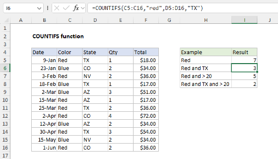
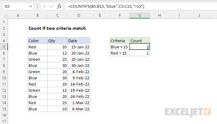
To count rows where two (or more) criteria match, you can use a formula based on the COUNTIFS function. In the example shown, the formula in cell G5 is:
=COUNTIFS(B5:B15,"blue",C5:C15,">15")
The result is 3, since there are three rows with a color of "blue" and quantity greater than 15.
Generic formula
=COUNTIFS(range1,"blue",range2,">15")
Explanation
In this example, the goal is to count orders where the color is "blue" and the quantity is greater than 15. All data is in the range B5:B15. There are two primary ways to solve this problem, one with the COUNTIFS function, the other with the SUMPRODUCT function. Both approaches are explained below.
COUNTIFS function
The COUNTIFS function returns the count of cells that meet one or more criteria. COUNTIFS can be used with criteria based on dates, numbers, text, and other conditions. COUNTIFS supports logical operators (>,<,<>,=) and wildcards (*,?) for partial matching.
In this example, we want to count orders where the color is "blue" in column B and the quantity is greater than 15 in column C. The COUNTIFS function takes multiple criteria in pairs — each pair contains one range and the associated criteria for that range. To start off, we can write a formula like this to count orders where the color is "blue":
=COUNTIFS(B5:B15,"blue") // returns 5
COUNTIFS returns 5 since there are five cells in B5:B15 equal to "blue". Notice we have single range/criteria pair at this point. To add a condition to check for a quantity greater than (>) 15, we add another range/criteria pair like this:
=COUNTIFS(B5:B15,"blue",C5:C15,">15") // returns 3
This is the formula used in cell G5 in the example. COUNTIFS returns 3, since there are three rows in the data where the color in B5:B15 is "blue" and the quantity in C5:C15 is greater than 15. To generate a count, all conditions must match. To add more conditions, add more range/criteria pairs. For reference, the formula in G6 is:
=COUNTIFS(B5:B15,"red",C5:C15,">15") // returns 1
This time, COUNTIFS returns 1, since there is just one "red" order over 15.
SUMPRODUCT alternative
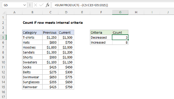
You can also use the SUMPRODUCT function to count rows that match multiple conditions. the equivalent formula is:
=SUMPRODUCT((B5:B15="blue")*(C5:C15>15)) // returns 3
This is an example of using Boolean logic in a formula. The first expression tests for "blue":
B5:B15="blue"
Because there are 11 cells in B5:B15, the expression returns 11 TRUE and FALSE values in an array like this:
{FALSE;TRUE;FALSE;TRUE;FALSE;TRUE;FALSE;FALSE;TRUE;FALSE;TRUE}
The second expression tests for a quantity greater than 15:
C5:C15>15
Because there are again 11 cells in C5:C15, this expression returns an array like this:
{FALSE;TRUE;FALSE;TRUE;FALSE;TRUE;FALSE;FALSE;TRUE;FALSE;TRUE}
The math operation of multiplying these two arrays together converts the TRUE and FALSE values to 1s and 0s:
=SUMPRODUCT({0;1;0;1;0;1;0;0;1;0;1}*{0;0;1;1;1;1;0;0;1;1;0})
After multiplication, we have a single array like this:
=SUMPRODUCT({0;0;0;1;0;1;0;0;1;0;0})
With just one array to process, SUMPRODUCT returns the sum, 3, as a final result.
SUMPRODUCT is more powerful and flexible than COUNTIFS, which is in a group of eight functions require ranges. For more details, see Why SUMPRODUCT?.
Pivot table alternative
To summarize different combinations in a larger data set, consider a Pivot Table. Pivot tables are a fast and flexible reporting tool that can summarize data in many different ways. For a direct comparison of SUMIF and Pivot tables, see this video.