Excel formula: Conditional formatting based on another column

Generic formula

=$B1>$A1

Summary

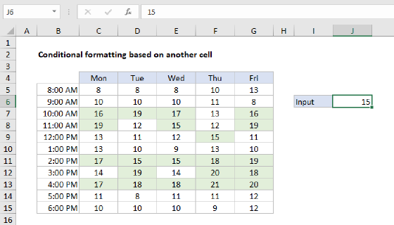
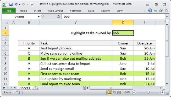
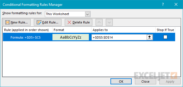
To apply conditional formatting based on a value in another column, you can create a rule based on a simple formula. In the example shown, the formula used to apply conditional formatting to the range D5:D14 is:

=$D5>$C5

This highlights values in D5:D14 that are greater than C5:C14. Note that both references are mixed in order to lock the column but allow the row to change.

Explanation

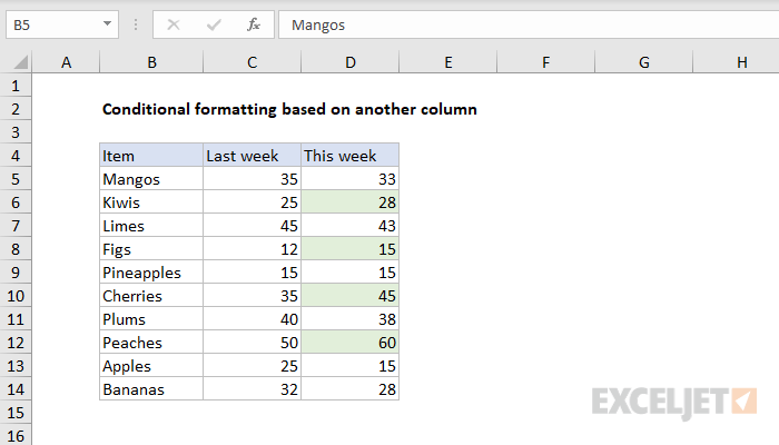
In this example, a conditional formatting rule highlights cells in the range D5:D14 when the value is greater than corresponding values in C5:C14. The formula used to create the rule is:

=$D5>$C5

The rule is applied to the entire range D5:G14. The formula uses the greater than operator (>) to evaluate each cell in D5:D14 against the corresponding cell in C5:C14. When the formula returns TRUE, the rule is triggered and the highlighting is applied.

Conditional formatting rule applied to D5:D14

Mixed references

The mixed references used in this formula ($D5, $C5) make this rule portable. You could use the same formula to highlight cells in B5:B14 instead of D5:D14, or even to highlight entire rows based on the same logic.

Quick Start | More Examples | Troubleshooting | Training

Author

Dave Bruns

Related formulas

Conditional formatting based on another cell

Excel contains many built-in "presets" for highlighting values with conditional formatting, including a preset to highlight cells greater than a specific value. However, by using your own formula, you have more flexibility and control. In this...

Highlight values between

When you use a formula to apply conditional formatting, the formula is evaluated for each cell in the range, relative to the active cell in the selection at the time the rule is created. So, in this case, if you apply the rule to B4:G11, with B4 as...

Highlight values greater than

When you use a formula to apply conditional formatting, the formula is evaluated relative to the active cell in the selection at the time the rule is created. So, in this case the formula =B4>100 is evaluated for each of the 40 cells in B4:G11...

Highlight cells that contain

When you use a formula to apply conditional formatting, the formula is evaluated relative to the active cell in the selection at the time the rule is created. In this case, the rule is evaluated for each of the 10 cells in B2:B11, and B2 will change...

Highlight entire rows

When you use a formula to apply conditional formatting, the formula is evaluated relative to the active cell in the selection at the time the rule is created. In this case, the address of the active cell (B5) is used for the row (5) and entered as a...

Related videos

How to apply conditional formatting with a formula

In this video, we'll look at how to use a simple formula to apply conditional formatting. Formulas allow you to create more flexible and powerful conditional formats.

Conditional formatting based on a different cell

In this video, we'll look at how to apply conditional formatting to one cell based on values in another, using a formula.

How to build a search box with conditional formatting

In this video, we'll look at a way to create a search box that highlights rows in a table, by using conditional formatting, and a formula that checks several columns at once.

How to highlight rows with conditional formatting

In this video, we'll show you how to use a formula with conditional formatting to highlight an entire row in a multi-column list.

How to create a mixed reference

In this video, we look at how to create a mixed reference that is part relative, and part absolute, useful when you want only part of a cell reference to change.

Excel Formula Training

Formulas are the key to getting things done in Excel. In this accelerated training, you'll learn how to use formulas to manipulate text, work with dates and times, lookup values with VLOOKUP and INDEX & MATCH, count and sum with criteria, dynamically rank values, and create dynamic ranges. You'll also learn how to troubleshoot, trace errors, and fix problems. Instant access. See details here.