=ISNA(value)- value - The value to check if #N/A.
Using the ISNA function
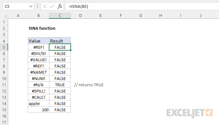
The ISNA function returns TRUE when a cell contains the #N/A error and FALSE for any other value, or any other error type. The ISNA function takes one argument, value, which is typically a cell reference.
Examples
If A1 contains the #N/A error, ISNA returns TRUE:
=ISNA(A1) // returns TRUE
ISNA returns FALSE for other values and errors:
=ISNA(100) // returns FALSE
=ISNA(5/0) // returns FALSE
You can use the ISNA function with the IF function test for #N/A and display a friendly message if the error occurs. For example, to display a message if A1 contains #N/A and the value of A1 if not:
=IF(ISNA(A1),"message",A1)
The IFNA function is a more efficient way to trap the #N/A error. See VLOOKUP without NA error for an example.
Return #N/A
To explicitly return the #N/A error in a formula, you can use the NA function:
=NA() // returns #N/A error
The following will return true:
=ISNA(NA()) // returns TRUE
Count #N/A errors
To count cells in a range that contain #N/A errors, you can use the SUMPRODUCT function like this:
=SUMPRODUCT(--ISNA(range))
The double negative coerces the TRUE and FALSE results from ISNA into 1s and 0s and SUMPRODUCT sums the result.
Notes
- The IFNA function is a more efficient way to trap and handle the #N/A error.