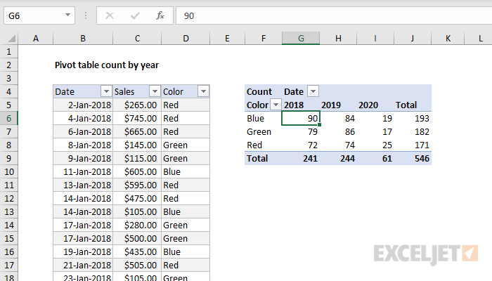
Pivot tables have a built-in feature to group dates by year, month, and quarter. In the example shown, a pivot table is used to count colors per year. This is the number of records that occur for each color in a given year.
Fields
The source data contains three fields: Date, Sales, and Color. Only two fields are used to create the pivot table: Date and Color.
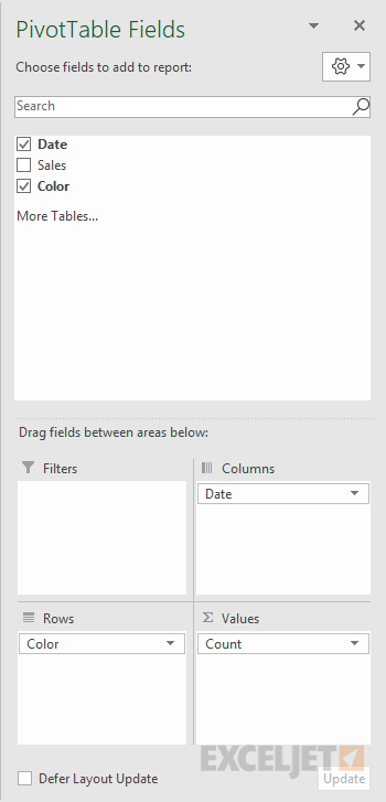
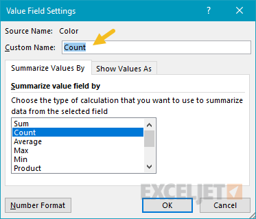
The Color field has been added as a Row field to group data by color. The Color field has also been added as a Value field, and renamed "Count":
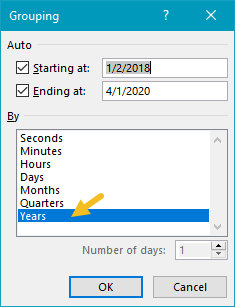
The Date field has been added as a Column field and grouped by year:
Helper column alternative
As an alternative to automatic date grouping, you can add a helper column to the source data, and use a formula to extract the year. Then add the Year field to the pivot table directly.
Steps
- Create a pivot table
- Add Color field to Rows area
- Add Color field Values area, rename to "Count"
- Add Date field to Columns area, group by Year
- Change value field settings to show count if needed
Notes
- Any non-blank field in the data can be used in the Values area to get a count.
- When a text field is added as a Value field, Excel will display a count automatically.
- Without a Row field, the count represents all data records.


