Explanation
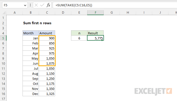
In the example shown, we have a list of amounts by month. The goal is to dynamically sum values through a given number of months using a variable n in cell E5. Since month names are just text, and months are listed in order, the key requirement is to sum amounts by position, starting with cell C5. In other words, we want to sum the first n values starting at cell C5. In the latest version of Excel, the best way to solve this problem is with the TAKE function, a new dynamic array function in Excel. In older versions of Excel, you can use the OFFSET function. Both approaches are explained below.
TAKE function
The TAKE function returns a subset of a given array. The number of rows and columns to return is provided by separate rows and columns arguments. For example, you can use TAKE to return the first 3 rows or columns of an array like this:
=TAKE(array,3) // first 3 rows
=TAKE(array,,3) // first 3 columns
In this problem, the values we want to sum are in the range C5:C16, and the number of rows to return is a variable entered in cell E5. To return the first n values from C5:C16, we use TAKE like this:
=TAKE(C5:C16,E5)
In this configuration, TAKE will return an array with six values like this:
{900;850;925;975;1050;1075}
To sum these values, we nest the TAKE function inside the SUM function like this:
=SUM(TAKE(C5:C16,E5))
=SUM({900;850;925;975;1050;1075})
=5775
The result is 5,775, the sum of the first six values in the range C5:C16.
OFFSET function
In older versions of Excel that do not have the TAKE function, you can use the OFFSET function to solve this problem. OFFSET is designed to create a reference to a range constructed using five inputs: (1) a starting point, (2) a row offset, (3) a column offset, (4) a height in rows, (5) a width in columns. To sum the first 6 values in C5:C16, we can use the OFFSET function with the SUM function like this:
=SUM(OFFSET(C5,0,0,E5))
Inside OFFSET, we use C5 for reference, since we want to start at C5. Next, we provide 0 for rows and 0 for cols since we don't want a row offset or a column offset. Finally, we provide E5 for height, since this cell contains the number of rows to include in the sum. We don't need to provide a value for the optional width argument, since width will be automatically inherited from reference. In this configuration, OFFSET will return a reference to C5:C10. The formula will evaluate like this:
=SUM(OFFSET(C5,0,0,E5))
=SUM(C5:C10)
=SUM({900;850;925;975;1050;1075})
=5775
The final result is 5,775, the sum of the first six values in the range C5:C16.


