Summary
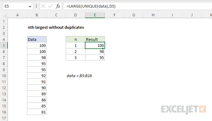
To get the nth largest value in a way that excludes duplicate values, you can use a formula based on the LARGE function and the UNIQUE function. In the worksheet shown, the formula in cell E5, copied down, is:
=LARGE(UNIQUE(data),D5)
where data is the named range B5:B16. As the formula is copied down, it returns the top 3 values in the data, which are 100, 98, and 95.
Note: UNIQUE is a newer function in Excel. See below for a formula that will work in older versions of Excel.
Generic formula
=LARGE(UNIQUE(range),n)
Explanation
In this example, the goal is to retrieve the largest 3 (top 3) values in the named range data, which appears in the range B6:B16. The standard solution to get "nth largest values" is the LARGE function. However, one potential problem with LARGE is that it will return duplicate values if they are present in the source data.
Named range
For convenience, all values are in the named range data (B6:B16). Using a named range is entirely optional, but it's a nice way to quickly try out a number of formulas without entering addresses and locking references.
Video: How to create a named range
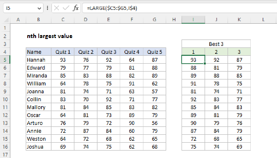
LARGE function
The LARGE function is used to return the nth largest value in a set of data like this:
=LARGE(range,n)
where n is a number like 1, 2, 3, etc. For example, you can retrieve the first, second, and third largest values like this:
=LARGE(range,1) // first largest
=LARGE(range,2) // second largest
=LARGE(range,3) // third largest
The challenge in this problem is that LARGE will return duplicates. For example, because 100 is the top value in the data and occurs twice, LARGE will return 100 when n = 1 and when n = 2.
LARGE with UNIQUE
One easy way to solve this problem is to use the UNIQUE function inside of LARGE. This is the approach seen in the worksheet shown, where the formula in cell E5 is:
=LARGE(UNIQUE(data),D5)
The UNIQUE function simply returns UNIQUE values, so the formula is solved like this:
=LARGE(UNIQUE(data),D5)
=LARGE(UNIQUE({100;100;98;95;95;92;91;90;89;86;85;81}),D5)
=LARGE({100;98;95;92;91;90;89;86;85;81},1)
=100
In cell E6 when n = 2, we get 98:
=LARGE(UNIQUE(data),D5)
=LARGE(UNIQUE({100;100;98;95;95;92;91;90;89;86;85;81}),D5)
=LARGE({100;98;95;92;91;90;89;86;85;81},2)
=98
Without the UNIQUE function, LARGE would return 100 when n = 2.
Legacy Excel
In older versions of Excel that do not have the UNIQUE function, we need a different approach. One option is to use the MAX function with the IF function. We start off with MAX alone in cell E5:
=MAX(data) // returns 100
MAX returns 100, the largest value in data. Next in cell E6, we enter a different formula that uses the IF function to "filter" out previous values like this:
=MAX(IF(data<E5,data))
Note: this is an array formula and must be entered with control + shift + enter in Legacy Excel.
This formula evaluates like this:
=MAX(IF(data<E5,data))
=MAX({FALSE;FALSE;98;95;95;92;91;90;89;86;85;81})
=98
Notice that the IF function converts the value of 100 (which occurs twice) to FALSE. In other words, values that have appeared previously are destroyed. The MAX function simply returns the maximum value in the remaining numbers. As the formula is copied down the column, the reference to E5 changes at each row and IF creates a new array that excludes the previous result, and MAX returns a new maximum value.