XLOOKUP wildcard contains substring

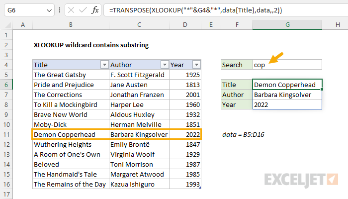
The goal is to look up the Title, Author, and Year in the list of books as shown using a formula based on a partial match and a wildcard. The text string to search for is entered in cell G4. All data is in an Excel Table named data in the range B5:D16. This problem can be easily solved with the XLOOKUP function or the VLOOKUP function. Both methods are explained below.

XLOOKUP function

The XLOOKUP function is a modern upgrade to the VLOOKUP function. The full generic syntax for XLOOKUP looks like this:

=XLOOKUP(lookup_value,lookup_array,return_array,if_not_found,match_mode,search_mode)

Briefly, these arguments have the following meaning:

• lookup_value - the value to look for
• lookup_array - the range or array to search within
• return_array - the range or array to return values from
• if_not_found - the value to return if the lookup_value is not found 
• match_mode - settings for exact, approximate, and wildcard matching
• search_mode - control for search direction, and binary search

The XLOOKUP function has built-in support for formula wildcards when the match_mode argument is set to 2. Only the first three arguments are required in XLOOKUP so for this problem we need to supply four values: lookup_value, lookup_array, return_array, and match_mode:

=XLOOKUP(lookup_value,lookup_array,return_array,,match_mode)

Notice that we simply leave if_not_found empty, though you are free to enter any value you like here. To start off, we provide lookup_value. This is the tricky part of the formula:

=XLOOKUP("*"&G4&"*",

Here, we concatenate the value in cell G4 to with an asterisk (*) wildcard on either side. With the string "cop" in cell G4, the result will be a string like "*cop*".The asterisk will match "zero or more characters" so by using an asterisk at the start and the end of the search string, we are asking XLOOKUP to match the text anywhere it occurs in the Title, which is provided as lookup_array:

XLOOKUP("*"&G4&"*",data[Title],

Next, we need to provide the return_array. Here, because we want all three columns of data, we use another small trick. Instead of asking for each column separately, we ask for the entire table, which is named data:

XLOOKUP("*"&G4&"*",data[Title],data,

This will cause XLOOKUP to return the entire matching row, with Title, Author, and Year included. Next, we omit a value for if_not_found by simply skipping the argument altogether. Feel free to use a value like "Not found" if you like.

XLOOKUP("*"&G4&"*",data[Title],data,,

Last, we need to provide a value for match_mode. To enable wildcard matching with XLOOKUP, supply the number 2. This is the final XLOOKUP formula in cell G6:

XLOOKUP("*"&G4&"*",data[Title],data,,2)

There is one more step we need to take. Because we have asked XLOOKUP to return the entire matching row, XLOOKUP will return three values (Title, Author, and Year) in an array that spills onto the worksheet in the original horizontal orientation. We need the results to be organized vertically, so we nest the XLOOKUP function inside the TRANSPOSE function like this:

=TRANSPOSE(XLOOKUP("*"&G4&"*",data[Title],data,,2))

Transpose will "flip" the orientation of the array returned by XLOOKUP. With the text "cop" in cell G4, XLOOKUP will return an array to the TRANSPOSE funtion like this:

=TRANSPOSE({"Demon Copperhead","Barbara Kingsolver",2022})

The comma separators tell us this is a horizontal array. After TRANSPOSE runs, we have an array like this:

{"Demon Copperhead";"Barbara Kingsolver";2022}

The semicolons (;) indicate a vertical array. The array lands in cell G6, and the values spill vertically into the range G6:G8.

XLOOKUP with individual columns

Although the formula used in the worksheet has XLOOKUP set to return an entire row from data, we can easily configure XLOOKUP to return individual columns like this:

=XLOOKUP("*"&G4&"*",data[Title],data[Title],,2) // title
=XLOOKUP("*"&G4&"*",data[Title],data[Author],,2) // author
=XLOOKUP("*"&G4&"*",data[Title],data[Year],,2) // year

Because each formula outputs a single value, the formulas can be placed in any cell and there is no need for the TRANSPOSE function. 

Get all matches

If you want to get all matches, instead of the first match, you will need to use the FILTER function. You can find an example of FILTER with a "text contains" type match here.

VLOOKUP function

In older versions of Excel that do not offer the XLOOKUP function, the VLOOKUP function can be used instead like this:

=VLOOKUP("*"&G4&"*",data,1,0) // title
=VLOOKUP("*"&G4&"*",data,2,0) // author
=VLOOKUP("*"&G4&"*",data,3,0) // year

For lookup_value, we use the same wildcard trick explained above: we concatenate an asterisk (*) to either side of the search string in G4:

=VLOOKUP("*"&G4&"*",

For table_array, we provide the Excel Table named data:

=VLOOKUP("*"&G4&"*",data,

Next, we need to supply a column number, where Title = 1, Author = 2, and Year = 3. To retrieve the Title, we provide 1 for col_index_num:

=VLOOKUP("*"&G4&"*",data,1

Finally, we must set VLOOKUP in exact match mode to enable wildcard support. To do that, we provide FALSE or zero for the last argument, called range_lookup, like this:

=VLOOKUP("*"&G4&"*",data,1,0)

The formulas to retrieve Author and Year are the same, except for the column number:

=VLOOKUP("*"&G4&"*",data,2,0) // author
=VLOOKUP("*"&G4&"*",data,3,0) // year