Summary
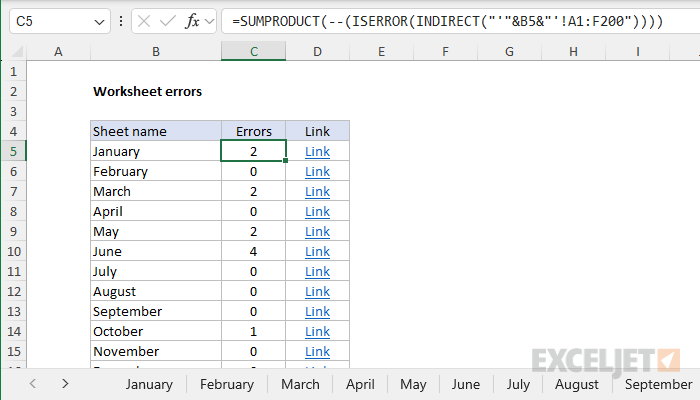
To count errors by sheet a workbook you can use a formula based on the ISERROR function, with help from INDIRECT and SUMPRODUCT. In the worksheet shown, the formula in cell C5 is:
=SUMPRODUCT(--(ISERROR(INDIRECT("'"&B5&"'!A1:F101"))))
As the formula is copied down, it returns a count of errors on each worksheet listed in column B. See below for options to generate a list of sheet names automatically.
Generic formula
=SUMPRODUCT(--(ISERROR(INDIRECT("'"&A1&"'!range"))))
Explanation
In this example, the goal is to count errors in a workbook by sheet, where the sheet names have been previously entered in a column as shown. This is a tricky problem in Excel for a couple of reasons. First, there is no direct way to generate a list of sheets in a workbook with a formula. Second, once we have a list of sheet names, we need to run the text through the INDIRECT function to get a valid reference. Nevertheless, this is an interesting problem that provides a useful way to audit sheets in a workbook for errors. The article below explains the steps needed to create the report, and options for generating a list of sheet names.
Note: INDIRECT is a volatile function that can cause performance problems in large or complex workbooks.
Step 1: Create a new sheet to track errors
The first step is to create a new sheet where you can enter the formulas needed to count errors. Create a new sheet using the "Plus" icon at the right of the existing sheets, then name the sheet "Errors". I recommend you place this sheet at the end of the workbook. In the example above, the Errors sheet is the last. You'll then want to format a column to hold the sheet names and error counts as seen in the example. Next, we need to create a list of sheet names.
Step 2: Create the list of sheet names
The next step is to create a list of sheet names. As mentioned above, there is no direct way to create a list of sheet names with a formula in Excel. The four main options are as follows:
- Enter the sheet names manually.
- Use a defined name + a formula (see below).
- Use Power Query (see below).
- Use VBA (not discussed in this article).
Before you try options #2 or #3 above, I recommend you enter a few sheet names manually and try out the formula to count errors on each sheet. It's a good idea to make sure the solution will be useful to you before investing more time.
Manual option
In a basic workbook, is it easy to manually create a list of sheet names with copy and paste:
- Double-click a sheet to select the name
- Copy the name to the clipboard (Control + C)
- Paste the name into a cell on the Errors sheet.
Repeat this process for each sheet in the workbook you want to track. Note that the names you enter must match the sheet names exactly. If you rename or add a new sheet, you will need to update the list of sheet names to match. If you are working with a large workbook with many sheets, this process can become tedious, and you may want to try a more automated solution to list sheet names. Here are two options:
Excel formula + defined name
One option is to create a defined name that refers to an Excel 4.0 macro, and then refer to the name in a regular formula. This option works pretty well and has the advantage of automatically updating the list of sheet names when there are changes. One disadvantage of this approach is that you will need to save the file as a macro-enabled workbook (.xlsm) if you want the sheet names to remain dynamic. For step-by-step instructions for listing sheet names with a formula, see this article.
Power Query
Another option to automatically generate sheet names in a workbook is to use Power Query. This is a more modern approach, and it works well, but the list of sheets won't automatically update when there are changes. Instead, you must right-click the list and click "Refresh". On the plus side, there is no need to save the file in a special format. See step-by-step instructions here.
Step 3: Enter a formula to count errors by sheet
Finally, we arrive at the point where we can count errors on each sheet. In the worksheet shown, the formula used to do this looks like this:
=SUMPRODUCT(--(ISERROR(INDIRECT("'"&B5&"'!A1:F200"))))
Note: we are hardcoding the range as A1:F200 which is big enough for the workbook in this example. You will need to adjust this range to suit your workbook. The range should be big enough to include the cells you care about on each sheet, but not so large as to cause performance problems in larger workbooks with many sheets. INDIRECT will trigger a recalculation with each change to the workbook!
Working from the inside out, the first step is to create a valid reference to a range on a sheet. This is done with the INDIRECT function, which is designed to convert a text string into a valid reference. For example:
=INDIRECT("A1") // returns a reference to A1
=INDIRECT("C5") // returns a reference to C5
=INDIRECT("Sheet1!A1:A10") // returns a reference to A1:A10 on Sheet1
The main thing to understand is each reference above begins as plain text. INDIRECT evaluates the text and converts it to a valid cell reference that can be used in a formula. In this example, INDIRECT is configured like this:
INDIRECT("'"&B5&"'!A1:F200")
The sheet name ("January") comes from cell B5. Inside INDIRECT, we are concatenating separate values into a single text string that can be interpreted as a range on the given sheet. Note we are carefully adding single quotes (') around the sheet name. These are required when a sheet name contains space or punctuation. We also need to add an exclamation point (!) before the range. After the individual values are joined into a single text string, the result looks like this:
INDIRECT("'January'!A1:F200")
INDIRECT then converts this text value into a valid reference and we now have a standard reference:
=SUMPRODUCT(--(ISERROR('January'!A1:F200)))
The next step is to count errors. First, we run the ISERROR function on all cells in the range A1:F200 on the January sheet:
ISERROR('January'!A1:F200)
ISERROR returns TRUE when a cell contains an error, and FALSE if not. Because there are 1200 cells in the range A1:F200, ISERROR returns an array that contains 1200 TRUE or FALSE results. Most of these values will be FALSE, since most cells in the range do not contain errors. Next, we use a double negative (--) on the result from ISERROR:
--(ISERROR('January'!A1:F200))
The only purpose of this operation is to convert the 1200 TRUE and FALSE values into 1s and 0s. After this step, the vast majority of the values will be zeros.
This is why we don't want to use an unnecessarily large range - we are asking Excel to perform a lot of calculations for each sheet, and because INDIRECT is a volatile calculation, these calculations will occur every time the worksheet is changed.
Finally, we are ready to add things up with the SUMPRODUCT function. SUMPRODUCT sums the values in the array (again, the majority of the values are zeros) and returns a total sum. This sum represents the count of errors on the sheet. As the formula is copied down, the same process is repeated for each sheet in the list.
Note: in Excel 2021 and later, you can replace the SUMPRODUCT function with the SUM function in this formula without special handling. In older versions, SUM must be entered as an array formula with control + shift + enter. See Why SUMPRODUCT? for more info.
Step 4: Add a link to each sheet (optional)
It is also possible to add a link to each worksheet with the HYPERLINK function. The formula in cell D5, copied down, is:
=HYPERLINK("#'"&B5&"'!B5","Link")
HYPERLINK takes two arguments: link_location and friendly_name. Link_location is the destination or path the link should follow, entered as a text value. Friendly_name is the anchor text that will be displayed with the link. One interesting feature of HYPERLINK is that it is programmed to evaluate text as a reference, so we don't need to use the INDIRECT in this formula. As before we are concatenating values together to assemble a reference to a particular sheet. the only difference is that we add a hash character (#) at the start, which is required by HYPERLINK when linking to a sheet. After concatenation, we have the following:
=HYPERLINK("#'January'!B5","Link")
The result is a clickable link to cell B5 on the "January" sheet. As the formula is copied down, it returns a link to each sheet in the list. You can customize the destination cell and the anchor text as desired.
Tip: On a sheet with errors, you can select all errors with Go To (Control + G) > Formulas > Errors
Step 5: Trap errors (optional)
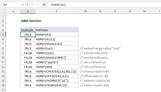
If a sheet name is not valid, INDIRECT will return a #REF error. Normally, we might see this error on the worksheet, but because we are nesting INDIRECT inside ISERROR, ISERROR will see the #REF error and return TRUE, causing the formula to return a count of 1. This is misleading because the error is not on the target sheet but instead a problem with the reference itself. One way to trap this error is to check the reference returned by INDIRECT first like this:
=IF(ISREF(INDIRECT("'"&B5&"'!A1:F200")),SUMPRODUCT(--(ISERROR(INDIRECT("'"&B5&"'!A1:F200")))),"Invalid reference")
Translation: If the reference returned by INDIRECT is valid, run the original formula. Otherwise, return "Invalid reference".
The ISREF function is used to test the reference returned by INDIRECT and the IF function is used to control the flow. In a newer version of Excel you can clean things up a bit by adding the LET function and running INDIRECT just once like this:
=LET(
ref,INDIRECT("'"&B5&"'!A1:F200"),
IF(ISREF(ref),SUMPRODUCT(--ISERROR(ref)),"Invalid reference")
)