Summary
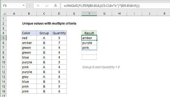
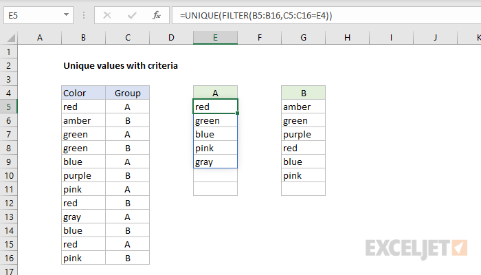
To extract a list of unique values from a set of data, while applying one or more logical criteria, you can use the UNIQUE function together with the FILTER function. In the example shown, the formula in D5 is:
=UNIQUE(FILTER(B5:B16,C5:C16=E4))
which returns the 5 unique values in group A, as seen in E5:E9.
Generic formula
=UNIQUE(FILTER(rng1,rng2=A1))
Explanation
This example uses the UNIQUE function together with the FILTER function. Working from the inside out, the FILTER function is first used to remove limit data to values associated with group A only:
FILTER(B5:B16,C5:C16=E4)
Notice we are picking up the value "A" directly from the header in cell E4. Insider filter the expression C5:C16=E4 returns an array of TRUE FALSE values like this:
{TRUE;FALSE;TRUE;FALSE;TRUE;FALSE;TRUE;FALSE;TRUE;FALSE;TRUE;FALSE}
This array is used to filter data, and the FILTER function returns another array as a result:
{"red";"amber";"green";"green";"blue";"pink";"red";"blue";"amber"}
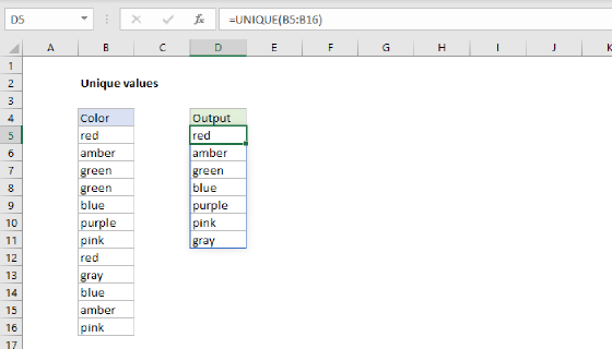
This array is returned directly to the UNIQUE function as the array argument. UNIQUE then removes duplicates, and returns the final array:
{"red";"green";"blue";"pink";"gray"}
UNIQUE and FILTER are dynamic functions. If data in B5:B16 or C5:C16 changes, the output will update immediately.
The formula in G5, which returns unique values associated with group B, is almost the same:
=UNIQUE(FILTER(B5:B16,C5:C16=G4))
The only difference is that C5:C16 is compared to the value in G4, which is "B".
Dynamic source range
Because ranges B5:B15 and C5:C16 are hardcoded directly into the formula, they won't resize if data is added or deleted. To use a dynamic range that will automatically resize when needed, you can use an Excel Table, or create a dynamic named range with a formula.
Dynamic Array Formulas are available in Office 365 only.