Translate letters to numbers

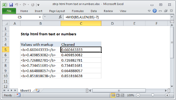
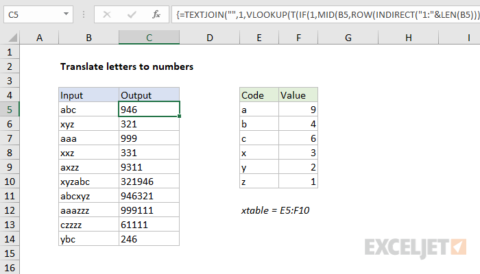
To translate letters in a string to numbers, you can use an array formula based on the TEXTJOIN and VLOOKUP functions, with a defined translation table to provide the necessary lookups. In the example shown, the formula in C5 is:

{=TEXTJOIN("",1,VLOOKUP(T(IF(1,MID(B5,ROW(INDIRECT("1:"&LEN(B5))),1))),xtable,2,0))}

where "xtable" is the named range E5:F10.

Note: this is an array formula and must be entered with control + shift + enter.

How this formula works

At the core, this formula uses an array operation to generate an array of letters from the input text, translates each letter individually to a number, then joins all numbers together again and returns the output as a string.

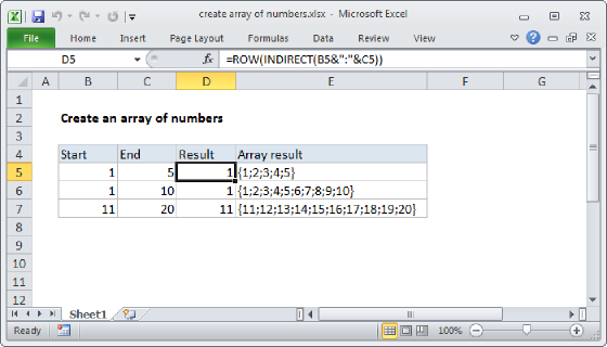
To parse the input string into an array or letters, we use MID, ROW, LEN and INDIRECT functions like this:

MID(B5,ROW(INDIRECT("1:"&LEN(B5))),1)

LEN returns the length of the input text, which is concatenated to "1:" and handed off to INDIRECT as text. INDIRECT evaluates the text as a row reference, and the ROW function returns an array of numbers to MID:

MID(B5,{1;2;3},1)

MID then extracts one character for at each starting position and we have:

=TEXTJOIN("",1,VLOOKUP(T(IF(1,{"a";"b";"c"})),xtable,2,0))

Essentially, we are asking VLOOKUP to find a match for "a", "b", and "c" at the same time. For obscure reasons, we need to "dereference" this array in a particular way using both the T and IF functions. After VLOOKUP runs, we have:

=TEXTJOIN("",1,{9;4;6})

and TEXTJOIN returns the string "946".

Output a number

To output a number as final result (instead of a string), add zero. The math operation will coerce the string into a number.

Sum numbers

To sum the numbers together instead of listing them, you can replace TEXTJOIN with SUM like this:

=SUM(VLOOKUP(T(IF(1,MID(B5,ROW(INDIRECT("1:"&LEN(B5))),1))),xtable,2,0))

Note: the TEXTJOIN function was introduced via the Office 365 subscription program in 2018.