Summary
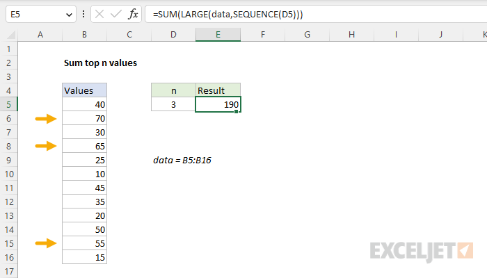
To sum the largest n values in a range, you can use a formula based on the LARGE function. In the example shown, the formula in cell E5 is:
=SUM(LARGE(data,SEQUENCE(D5)))
where data is the named range B5:B16. The result 190, the sum of 70, 65, and 55.
Generic formula
=SUM(LARGE(range,SEQUENCE(n)))
Explanation
In this example, the goal is to sum the largest n values in a set of data, where n is a variable that can be easily changed. For convenience, the range B5:B16 is named data. At a high level, the solution breaks down into two steps: (1) extract the n largest values from the data set and (2) sum the extracted values. There are several ways to approach this problem depending on what version of Excel is available. Regardless of the approach, all solutions below depend on the LARGE function.
LARGE function
The LARGE function is designed to return the nth largest value in a range. For example:
=LARGE(range,1) // 1st largest
=LARGE(range,2) // 2nd largest
=LARGE(range,3) // 3rd largest
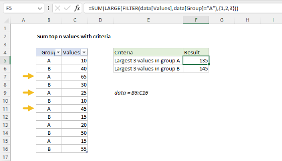
Normally, LARGE returns just one value. However, if you supply an array like {1,2,3} to LARGE as the second argument, k , LARGE will return an array of results instead of a single result. For example, the formula below will return the 3 largest values in B5:B16:
=LARGE(data,{1,2,3}) // returns {70;65;55}
Note that the result from LARGE is an array. By nesting the LARGE function side the SUM function, we can get a sum of the 3 largest three values in data:
=SUM(LARGE(data,{1,2,3})) // returns 190
The SUM function returns a result of 190, the sum of 70, 65, and 55. In older versions of Excel, you might have to use the SUMPRODUCT function instead of the SUM function, for reasons described here.
Given the formula outlined above, the challenge becomes how best to create the array needed to extract the top n values from a set of data. This depends on what Excel version is available.
Current Excel
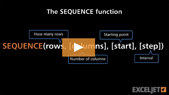
The latest version of Excel supports dynamic array formulas and provides a number of functions that make working with arrays easier. One of these functions is SEQUENCE, which is designed to generate arrays on the fly. In the example shown, the formula in E5 uses SEQUENCE to create a numeric array based on the value for n in cell D5
=SUM(LARGE(data,SEQUENCE(D5)))
Working from the inside out, the SEQUENCE function is configured with the rows argument set to cell D5. With the number 3 in D5, sequence generates a sequential array like this:
SEQUENCE(D5) // returns {1;2;3}
The numeric array is returned directly to the LARGE function for the k argument:
=SUM(LARGE(data,{1;2;3}))
And the solution proceeds as outlined above:
=SUM(LARGE(data,{1;2;3}))
=SUM({70;65;55})
=190
The final result is 190, as shown in the worksheet above.
Legacy Excel
In older versions of Excel that do not provide dynamic array support, or the SEQUENCE function, we need to take a different approach. One simple solution is to hardcode the numeric array given to LARGE as an array constant and switch to the SUMPRODUCT function:
=SUMPRODUCT(LARGE(data,{1,2,3}))
This formula works fine in older versions of Excel, but because the array is hardcoded inside LARGE, it is not a dynamic solution that uses the value for n in cell D5. In addition, as n becomes larger, it gets tedious to enter longer array constants like {1,2,3,4,5,6,7,8,9}, etc. To workaround this problem, you can use the more advanced formula below.
Dynamic n
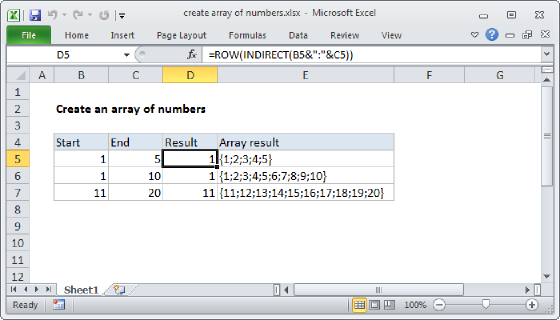
The classic solution for creating a numeric array in older versions of Excel is to use the ROW and INDIRECT functions. For example, to generate a numeric array from 1 to 10, you can use a formula like this:
=ROW(INDIRECT("1:10")) // returns {1;2;3;4;5;6;7;8;9;10}
The INDIRECT function converts the text string "1:10" to the range 1:10, which is returned to the ROW function. The ROW function returns the 10 row numbers that correspond to 1:10 in an array like this:
{1;2;3;4;5;6;7;8;9;10}
Note this is actually a vertical array, as indicated by the semicolons (;) but the LARGE function will happily accept a vertical or horizontal array for k. To adapt this approach in the worksheet as shown, we need to adjust the formula to concatenate the value for n to the string "1:" inside of INDIRECT like this:
=SUMPRODUCT(LARGE(data,ROW(INDIRECT("1:"&D5))))
This formula is now dynamic. When the value for n is changed, ROW and INDIRECT will spin up a new array that reflects the current value, and LARGE will extract the top n values as before, and SUMPRODUCT will return a sum.