Summary
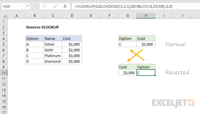
To reverse a VLOOKUP – i.e. to find the original lookup value using a VLOOKUP formula result – you can use a tricky formula based on the CHOOSE function, or more straightforward formulas based on INDEX and MATCH or XLOOKUP as explained below. In the example shown, the formula in H10 is:
=VLOOKUP(G10,CHOOSE({3,2,1},B5:B8,C5:C8,D5:D8),3,0)
With this setup, VLOOKUP finds the option associated with a cost of 3000, and returns "C".
Note: this is a more advanced topic. If you are just getting started with VLOOKUP, start here.
Generic formula
=VLOOKUP(A1,CHOOSE({3,2,1},col1,col2,col3),3,0)
Explanation
Introduction
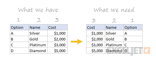
A key limitation of VLOOKUP is it can only look up values to the right. In other words, the column with lookup values must be to the left of the values you want to retrieve with VLOOKUP. As a result, with standard configuration, there is no way to use VLOOKUP to "look left" and reverse the original lookup. From the standpoint of VLOOKUP, we can visualize the problem like this:
The workaround explained below uses the CHOOSE function to rearrange the table inside VLOOKUP. Starting at the beginning, the formula in H5 is a normal VLOOKUP formula:
=VLOOKUP(G5,B5:D8,3,0) // returns 3000
Using G5 as the lookup value ("C"), and the data in B5:D8 as the table array, VLOOKUP performs a lookup on values in column B and returns the corresponding value from column 3 (column D), 3000. Notice zero (0) is provided as the last argument to force an exact match.
The formula in G10 simply pulls the result from H5:
=H5 // 3000
To perform a reverse lookup, the formula in H10 is:
=VLOOKUP(G10,CHOOSE({3,2,1},B5:B8,C5:C8,D5:D8),3,0)
The tricky bit is the CHOOSE function, which is used to rearrange the table array so that Cost is the first column, and Option is the last:
CHOOSE({3,2,1},B5:B8,C5:C8,D5:D8) // reorder table 3, 2, 1
The CHOOSE function is designed to select a value based on a numeric index. In this case, we are supplying three index values in an array constant:
{3,2,1} // array constant
In other words, we are asking for column 3, then column 2, then column 1. This is followed by the three ranges that represent each column of the table in the order they appear on the worksheet.
With this configuration, CHOOSE returns all three columns in a single 2D array like this:
{1000,"Silver","A";2000,"Gold","B";3000,"Platinum","C";5000,"Diamond","D"}
If we visualize this array as a table on the worksheet, we have:
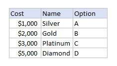
Note: the headings are not part of the array and are shown here for clarity only.
Effectively, we have swapped columns 1 and 3. The reorganized table is returned directly to VLOOKUP, which matches 3000, and returns the corresponding value from column 3, "C".
With INDEX and MATCH
The above solution works fine, but it is hard to recommend since most users will not understand how the formula works. A better solution is INDEX and MATCH, using a formula like this:
=INDEX(B5:B8,MATCH(G10,D5:D8,0))
Here, the MATCH function finds the value 3000 in D5:D8, and returns its position, 3:
MATCH(G10,D5:D8,0) // returns 3
Note: MATCH is configured for an exact match by setting the last argument to zero (0).
MATCH returns a result directly to INDEX as the row number, so the formula becomes:
=INDEX(B5:B8,3) // returns "C"
and INDEX returns the value from the third row of B5:B8, "C".
This formula shows how INDEX and MATCH can be more flexible than VLOOKUP.
With XLOOKUP
XLOOKUP also provides a very good solution. The equivalent formula is:
=XLOOKUP(G10,D5:D8,B5:B8) // returns "C"
With a lookup_value from G10 (3000), a lookup_array of D5:D8 (costs), and a results_array of B5:B8 (options), XLOOKUP locates the 3000 in the lookup array and returns the corresponding item from the results array, "C". Because XLOOKUP performs an exact match by default, there is no need to set the match mode explicitly.