Summary
To rank items in a list using one or more criteria, you can use the COUNTIFS function. In the example shown, the formula in E5 is:
=COUNTIFS(groups,C5,scores,">"&D5)+1
where "groups" is the named range C5:C14, and "scores" is the named range D5:D14. The result is a rank for each person in their own group.
Note: although data is sorted by group in the screenshot, the formula will work fine with unsorted data.
Generic formula
=COUNTIFS(criteria_range,criteria,values,">"&value)+1
Explanation
Although Excel has a RANK function, there is no RANKIF function to perform a conditional rank. However, you can easily create a conditional RANK with the COUNTIFS function.
The COUNTIFS function can perform a conditional count using two or more criteria. Criteria are entered in range/criteria pairs. In this case, the first criteria restricts the count to the same group, using the named range "groups" (C5:C14):
=COUNTIFS(groups,C5) // returns 5
By itself, this will return total group members in group "A", which is 5.
The second criteria restricts the count to only scores greater than the "current score" from D5:
=COUNTIFS(groups,C5,scores,">"&D5) // returns zero
The two criteria work together to count rows where the group is A and the score is higher. For the first name in the list (Hannah), there are no higher scores in group A, so COUNTIFS returns zero. In the next row (Edward), there are three scores in group A higher than 79, so COUNTIFS returns 3. And so on.
To get a proper rank, we simply add 1 to the number returned by COUNTIFS.
Reversing rank order
To reverse rank order and rank in order (i.e. smallest value is ranked #1) just use the less than operator (<) instead of greater than (>):
=COUNTIFS(groups,C5,scores,"<"&D5)+1
Instead of counting scores greater than D5, this version will count scores less than the value in D5, effectively reversing the rank order.
Duplicates
Like the RANK function, the formula on this page will assign duplicate values the same rank. For example, if a specific value is assigned a rank of 3, and there are two instances of the value in the data being ranked, both instances will receive a rank of 3, and the next rank assigned will be 5. To mimic the behavior of the RANK.AVG function, which would assign an average rank of 3.5 in such a case, you can calculate a "correction factor" with a formula like this:
=(COUNTIFS(groups,C5)+1-(COUNTIFS(group,C5,scores,">"&D5)+1)-(COUNTIFS(groups,C5,scores,"<"&D5)+1))/2
The result from this formula above can be added to the original rank to get an average rank. When a value has no duplicates, the above code returns zero and has no effect.