Summary
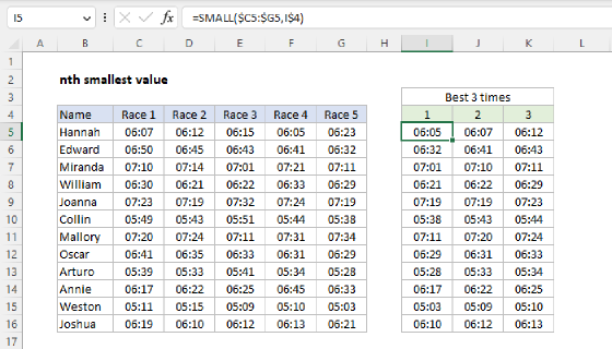
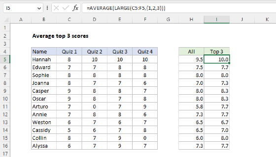
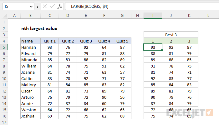
To get the nth largest value (i.e. 1st largest, 2nd largest, 3rd largest, etc.) in a set of data, you can use the LARGE function. In the example shown, the formula in I5 is:
=LARGE($C5:$G5,I$4)
As the formula is copied across and down the table, it returns the top 3 scores for each student in the list. Note this formula makes use of mixed references. See below for more information.
Generic formula
=LARGE(range,n)
Explanation
In this example, the goal is to extract the top 3 quiz scores for each name from the 5 scores that appear in columns C, D, E, F, and G. In other words, for each name listed, we want the best score, the 2nd best score, and the 3rd best score. This problem can be solved with the LARGE function.
Note: I don't know why the second argument for LARGE is called "k" . In this article I pretty much ignore that fact and use "n" instead, since "nth" is easier to understand than "kth".
LARGE function
The LARGE function can be used to return the nth largest value in a set of data. The generic syntax for LARGE looks like this:
=LARGE(range,n)
where n is a number like 1, 2, 3, etc. For example, you can retrieve the first, second, and third largest values like this:
=LARGE(range,1) // first largest
=LARGE(range,2) // second largest
=LARGE(range,3) // third largest
The LARGE function is fully automatic — you just need to supply a range and a number that indicates rank. The official names for these arguments are "array" and "k". To illustrate, below we use LARGE to get the top 3 scores in column C. The formula in F5, copied down, is:
=LARGE(data,E5)
Data is the named range C5:C16, provided as the array argument, and the value for k (n) comes from column E. As the formula is copied down, it returns the top 3 scores:
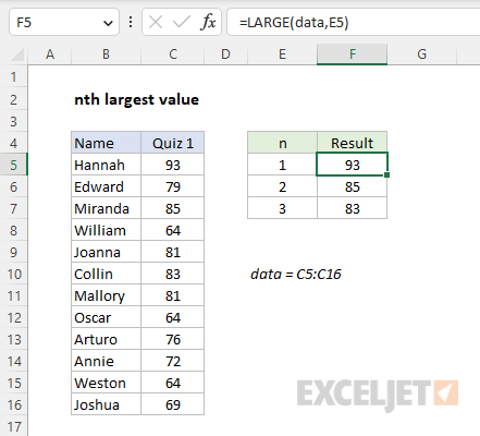
Here, data is the named range C5:C16, and the value for n comes from column E.
Mixed references
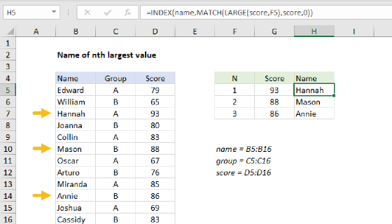
In the worksheet shown at top, we can use LARGE to get the top 3 scores for Hannah like this:
 =LARGE(C5:G5,1) // best score
 =LARGE(C5:G5,2) // 2nd best score
 =LARGE(C5:G5,3) // 3rd best score
The main challenge in this example is to create the syntax needed to copy the formula across the range I5:K16. In the example shown, this is accomplished with the formula in cell I5:
=LARGE($C5:$G5,I$4)
This is a clever use of mixed references that takes advantage of the fact that the numbers 1, 2, and 3 are already in the range I5:K5, so that they can be plugged into the formula directly as n:
- The value given for array is the mixed reference $C5:$G5. Notice that the columns are locked, but rows are not. This allows the rows to update as the formula is copied down, but prevents columns from changing as the formula is copied across.
- The value given for k (n) is another mixed reference, I$4. Here, the row is locked so that it will not change as the formula is copied down. However, the column is not locked, allowing it to change as the formula is copied across.