Summary
To list worksheets in an Excel workbook with a formula, you can use a 2-step approach: (1) define a named range called "sheetnames" with an old macro command and (2) use the TEXTAFTER function and the TRANSPOSE function to retrieve sheet names using the name. In the example shown, the formula in B5 is:
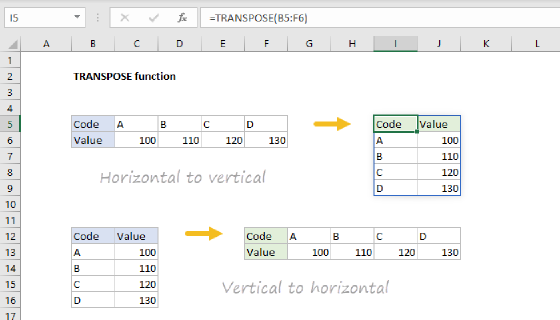
=TRANSPOSE(TEXTAFTER(sheetnames,"]"))
Notes: (1) In older versions of Excel without the TEXTAFTER function you can use a formula based on INDEX. See below for details (2) This article is about using Excel formulas to return a list of sheet names, but I've included a Power Query solution below as well.
Generic formula
=GET.WORKBOOK(1)&T(NOW())
Explanation
In this example, the goal is to generate a list of the sheet names in an Excel workbook with a formula. Unfortunately, there is no simple way to do this with a formula in Excel. However, it can be done with a two-step approach:
- Define a name called "sheetnames" with an old macro command and the Name Manager.
- Use the defined name in a formula that extracts the names into the workbook
The article below explains how to follow these steps. It includes a newer dynamic array formula that will return all sheets at once and a more traditional formula that will work in older versions of Excel.
This article is about using a formula to return a list of sheet names, but I've included a Power Query option below as well.
Step 1: Define the name
The first step is to define a new name. Navigate to the "Formulas" tab and click the "Define Name" button. In the "Name" field, enter "sheetnames". For the "Refers to" field, enter the formula below:
=GET.WORKBOOK(1)&T(NOW())
GET.WORKBOOK is part of a set of commands referred to as "Excel 4.0 macros" or "XLM macros," which were introduced with Excel 4 in the early 1990s. These macros provided basic automation in Excel before the introduction of Visual Basic for Applications (VBA) in Excel 5. This is essentially a hack that still works in later versions of Excel. In Excel 365, you might need to enable Excel 4.0 macros in the Trust Center, as explained below.
In the first part of the formula, GET.WORKBOOK(1), retrieves an array of sheet names in the current workbook. In a generic workbook called "workbook.xlsx" with five sheets, the resulting array looks like this:
{"[workbook.xlsx]Sheet1","[workbook.xlsx]Sheet2","[workbook.xlsx]Sheet3","[workbook.xlsx]Sheet4","[workbook.xlsx]Sheet5"}
Next, we concatenate a strange expression to the result:
&T(NOW())
I ran into this approach formula many years ago on the MrExcel message board in a post by T. Valko.
The purpose of this cryptic code is to trigger a recalculation when the worksheet changes. Since NOW is a volatile function, it will recalculate with each workbook change, like, for example, when a sheet is renamed. NOW returns a number indicating time in Excel, and the T function translates the number into an empty string (""). As a result, this part of the formula does not affect the output from GET.WORKBOOK; it is simply used to trigger recalculation.
Notes: (1) Because this step relies on a macro command, you'll need to save the file as a macro-enabled workbook (.xlsm) to allow the formula to update sheet names after the file is closed and re-opened. If you save the file as a normal worksheet (.xlsx), the sheetname code will be removed. (2) In newer versions of Excel, you may encounter a #BLOCKED error even after taking these steps. See below for a fix.
Step 2: enter a formula to retrieve sheet names
The second step in the process is to enter a formula that will retrieve the individual sheet names from the previously defined "sheetnames". In a modern version of Excel that provides dynamic array formulas and offers the TEXTAFTER function, you can use a formula like this to retrieve all sheet names in one step:
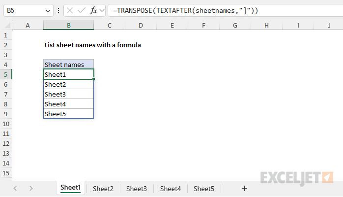
=TRANSPOSE(TEXTAFTER(sheetnames,"]"))
The TEXTAFTER function extracts just the sheet name from the full workbook path. The TRANSPOSE function converts the original horizontal array into a vertical array. The individual sheet names land in cell B5 and spill onto the worksheet. Done.
If you are using an older version of Excel without TEXTAFTER, see the next section.
Legacy formula
If you have an older version of Excel that does not support dynamic arrays, you will need to use a more traditional formula like this:
=INDEX(MID(sheetnames,FIND("]",sheetnames)+1,31),ROWS($B$5:B5))
Working from the inside out, the MID function is configured to extract each sheet name from the array returned by GET.WORKBOOK like this:
MID(sheetnames,FIND("]",sheetnames)+31)
The text argument is provided as sheetnames, which is the defined name created above. The value in sheetnames is an array like this:
{"[workbook.xlsx]Sheet1","[workbook.xlsx]Sheet2","[workbook.xlsx]Sheet3","[workbook.xlsx]Sheet4","[workbook.xlsx]Sheet5"}
The start_num argument is determined with the FIND function here:
FIND("]",sheetnames)+1
The FIND function locates the closing square bracket "]" in sheetnames, which appears right after the workbook name. The result is a number that indicates the position of this bracket. We add 1 because we want to start extracting the sheet name after the closing bracket. The value for num_chars is hardcoded as 31 to keep things simple. When num_chars exceeds the length of the text following the start number, MID returns all remaining text. Since sheet names cannot be longer than 31 characters, this ensures that we get the entire sheet name. The result from MID is an array like this:
{"Sheet1","Sheet2","Sheet3","Sheet4","Sheet5"}
At this point, we have the sheet names ready to go, we just need to get them onto the worksheet. We do this with the INDEX function. The array is delivered to INDEX as the array argument. The value for row_num is provided by the ROW function like this:
ROWS($B$5:B5)
The ROW function uses an expanding reference to generate an incrementing row number — as the formula is copied down, ROWS will return 1, then 2, then 3, etc. This allows INDEX to retrieve the next sheet name from the array at each new row. Copy the formula down until all sheet names are listed. When there are no more sheet names to output, the formula will return a #REF error.
Note: close observers will notice that we are asking INDEX for specific rows, even though the array is horizontal and has one row only. INDEX is clever this way — it knows what you want :)
Clearing a #BLOCKED error
In newer versions of Excel, you may run into a #BLOCKED error even after saving the file in .xlsm format and enabling VBA Macros. The error looks like this:
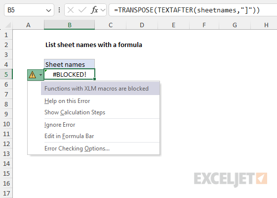
The problem occurs because a Trust Center setting called "Enable Excel 4.0 macros when VBA macros are enabled" in Excel 365 is disabled by default:
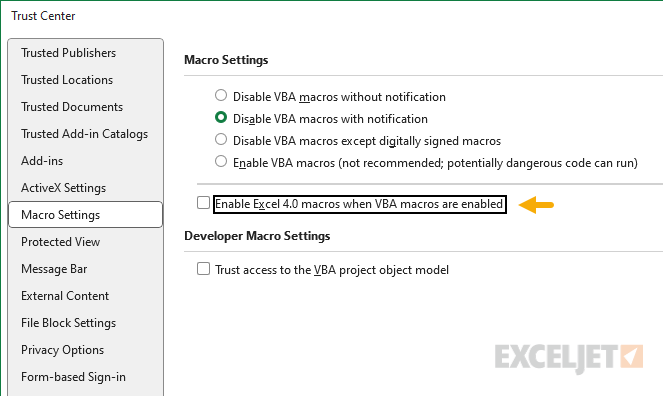
To open the Trust Center, navigate to File > Options > Trust Center, then click the "Trust Center Settings" button. To clear the blocked error, you will need to enable this setting. Check the checkbox and reopen the file. This time, when you are prompted to enable VBA macros the #BLOCKED error should be cleared.
List sheet names with Power Query
If you find the Macro-based solution above complex and underwhelming, there is another way to list sheet names in Excel: Power Query. Power Query is a heavy-duty data transformation tool, so this is a little like using a sledgehammer to crack a nut, but it works well. Below is a summary of the steps to list all Sheet names with Power Query. Don't be discouraged by the number of steps, you can do this in less than 2 minutes:
- Place your cursor in the cell where you want to list sheet names.
- Navigate to Data > Get Data > From File > From Excel Workbook.
- Select the current Excel workbook.
- Select any sheet name, then click the "Transform Data" button.
- Under Properties > Name, enter "List sheet names"
- Under Applied Steps, remove all steps except Source
- In the Kind column, filter to select "Sheet" only.
- Right-click the Name column and select "Remove other columns".
- Click "Close & Load" then select "Close & Load to"
- Select "Existing worksheet" and click "OK"
The sheet names will be delivered to the cell you selected in step #1 in an Excel table.
One disadvantage to the Power Query solution is that you must manually refresh the query if sheet names change — the list of sheet names won't automatically update. To refresh results, first save the workbook. Then Right-click the table and select "Refresh". One nice benefit of the Power Query approach is that you can easily exclude a sheet from the list. To exclude a specific sheet, click the filter button in the Name column after step #7 above then deselect the sheet(s) you want to exclude.
Notes: Power Query is built-in to Excel 2016 and later on Windows and is available as a free add-in for Excel 2010 and 2013. On the Mac, Power Query is available in Excel 365 but the feature set is more limited. The example above does work in a current version of Excel 365 on a Mac.