Summary
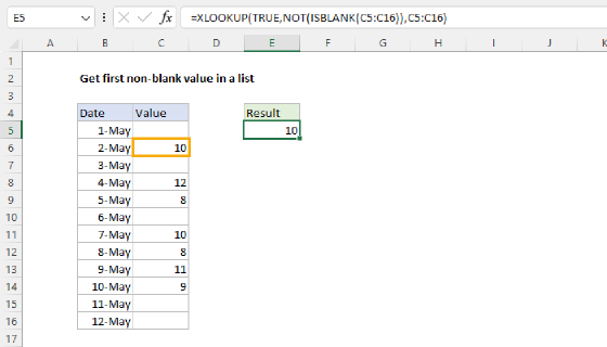
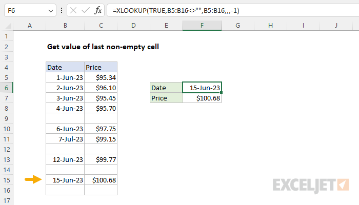
To get the value of the last non-empty cell in a range, you can use the XLOOKUP function. In the example shown, the formula in E5 is:
=XLOOKUP(TRUE,B5:B16<>"",B5:B16,,,-1)
The result is 15-Jun-23, as seen in cell B15. To get the corresponding amount in column C, just adjust the return_array, as explained below.
Generic formula
=XLOOKUP(TRUE,range<>"",range,,,-1)
Explanation
In this example, the goal is to get the last value in column B, even when data may contain empty cells. A secondary goal is to get the corresponding value in column C. This is useful for analyzing datasets where the most recent or last entry is significant. In the current version of Excel, a good way to solve this problem is with the XLOOKUP function. In older versions of Excel, you can use the LOOKUP function. Both methods are explained below.
XLOOKUP function
The XLOOKUP function is a modern upgrade to the VLOOKUP function. XLOOKUP is very flexible and can handle many different lookup scenarios. The key feature, in this case, is the ability to perform a "last to first" search. The generic syntax for XLOOKUP looks like this:
=XLOOKUP(lookup_value,lookup_array,return_array,if_not_found,match_mode,search_mode)
Where each argument has the following meaning:
- lookup_value - the value to look for
- lookup_array - the range or array to search within
- return_array - the range or array to return values from
- if_not_found - value to return if no match is found
- match_mode - settings for exact, approximate, and wildcard matching
- search_mode - settings for first to last, last to first, and binary searches
For more details, see How to use the XLOOKUP function.
In this example, we want to find the last non-empty cell in a range, so we use XLOOKUP like this:
=XLOOKUP(TRUE,B5:B16<>"",B5:B16,,,-1)
At a high level, we configure XLOOKUP to look for TRUE in a lookup array created with a logical expression, and we enable a "last to first" search by providing -1 for search_mode:
- lookup_value - TRUE
- lookup_array - B5:B16<>""
- return_array - B5:B16
- if_not_found - omitted, defaults to #N/A
- match_mode - omitted, defaults to exact match
- search_mode - given as -1 for search last to first
The main trick is the logical expression used for lookup_array:
B5:B16<>""
The <> operator means "not", so <>"" means "not empty". Because B5:B16 contains 12 values, the expression returns an array that contains 12 TRUE and FALSE results.
{TRUE;TRUE;TRUE;TRUE;FALSE;TRUE;TRUE;FALSE;TRUE;FALSE;TRUE;FALSE}
In this array, the TRUE values in the array indicate non-blank cells and the FALSE values indicate blank cells. This array is delivered directly to the XLOOKUP function as the lookup_array:
=XLOOKUP(TRUE,{TRUE;TRUE;TRUE;TRUE;FALSE;TRUE;TRUE;FALSE;TRUE;FALSE;TRUE;FALSE},B5:B16,,,-1)
Because search_mode is -1, XLOOKUP starts its search from the end of the array and matches the first TRUE encountered (the second to last value in the array). With the return_array provided as B5:B16, XLOOKUP returns 15-Jun-23 as a final result.
Corresponding value
The XLOOKUP formula in cell F7 to get the corresponding price from column C is almost identical:
=XLOOKUP(TRUE,B5:B16<>"",C5:C16,,,-1)
Note the only difference is the return_array, which is provided as C5:C16.
Dealing with errors
If the last non-empty cell contains an error, the error will be ignored. If you want to return an error that appears last in a range you can adjust the formula to use the ISBLANK and NOT functions like this:
=XLOOKUP(TRUE,NOT(ISBLANK(B5:B16)),B5:B16,,,-1)
This version of the formula will show an error if the last non-empty cell contains an error.
Last numeric value
To get the last numeric value, you can use the ISNUMBER function like this:
=XLOOKUP(TRUE,ISNUMBER(B5:B16),B5:B16,,,-1)
Last non-blank, non-zero value
To check that the last value is not blank and not zero, you use Boolean logic like this:
=XLOOKUP(1,(B5:B16<>"")*(B5:B16<>0),B5:B16,,,-1)
Notice the lookup value is now 1 instead of TRUE. For more details, see Boolean Algebra in Excel and XLOOKUP with multiple criteria.
Older versions of Excel
In older versions of Excel, there is no XLOOKUP function, so we need another approach. One solution is to use the LOOKUP function, which can handle array operations natively. The generic formula looks like this:
=LOOKUP(2,1/(range<>""),range)
Adjusting references for this problem, we have the following formula:
=LOOKUP(2,1/(B5:B16<>""),B5:B16)
Note: This is an array formula. But because LOOKUP can handle the array operation natively, the formula does not need to be entered with Control + Shift + Enter, even in older versions of Excel.
Working from the inside out, we use a logical expression to test for empty cells in B5:B16:
B5:B16<>""
The logical operator <> means not equal to, and "" means empty string, so this expression means B5:B16 is not empty. The result is an array of TRUE and FALSE values, where TRUE represents cells that are not empty and FALSE represents cells that are empty. Because B5:C16 contains 12 values, the expression returns an array with 12 results:
{TRUE;TRUE;TRUE;TRUE;FALSE;TRUE;TRUE;FALSE;TRUE;FALSE;TRUE;FALSE}
Next, we divide the number 1 by the array. The math operation automatically coerces TRUE to 1 and FALSE to 0, so we have:
1/({1;1;1;1;0;1;1;0;1;0;1;0})
Since dividing by zero generates an error, the result is an array composed of 1s and #DIV/0 errors:
{1;1;1;1;#DIV/0!;1;1;#DIV/0!;1;#DIV/0!;1;#DIV/0!}
Here, the 1s represent non-empty cells, and errors represent empty cells. This array becomes the lookup_array argument in LOOKUP. The lookup_value is given as the number 2. This may seem baffling, but there is a good reason. We are using 2 as a lookup value to force LOOKUP to scan to the end of the data. LOOKUP automatically ignores errors, so LOOKUP will scan through the 1s looking for a 2 that will never be found. When it reaches the end of the array, it will "step back" to the last 1, which corresponds to the last non-empty cell. Since the result_vector is B5:B16, the final result is: 15-Jun-23.
Note: the key to understanding this formula is to recognize that the lookup_value of 2 is deliberately larger than any values that will appear in the lookup_vector. When lookup_value can't be found, LOOKUP will match the next smallest value that is not an error: the last 1 in the array. This works because LOOKUP assumes that values in lookup_vector are sorted in ascending order and will always perform an approximate match. When LOOKUP can't find a match, it will match the next smallest value.
Get corresponding value
You can easily adapt the lookup formula to return a corresponding value. For example, to get the price associated with the last value in column B, the formula in F7 is:
=LOOKUP(2,1/(B5:B16<>""),C5:C16) // get price
The only difference is that the result_vector argument has been supplied as C5:C16.
Dealing with errors
If the last non-empty cell contains an error, the error will be ignored. If you want to return an error that appears last in a range you can adjust the formula to use the ISBLANK and NOT functions like this:
=LOOKUP(2,1/(NOT(ISBLANK(B5:B16))),B5:B16)
This version of the formula will show an error if the last non-empty cell contains an error.
Last numeric value
To get the last numeric value, you can use the ISNUMBER function like this:
=LOOKUP(2,1/(ISNUMBER(B5:B16)),B5:B16)
Last non-blank, non-zero value
To check that the last value is not blank and not zero, you can use Boolean logic like this:
=LOOKUP(2,1/((B5:B16<>"")*(B5:B16<>0)),B5:B16)
For a more detailed explanation, see Boolean Algebra in Excel.