Summary
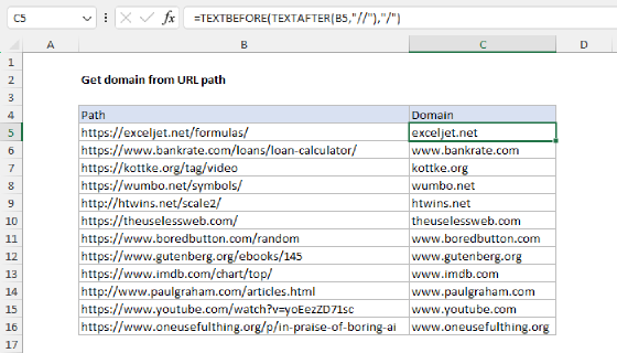
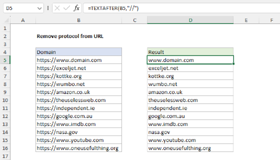
To extract the page from a URL (i.e. the part of a path after the domain), you can use a formula based on the TEXTAFTER function. In the example shown, the formula in D5 is:
="/"&TEXTAFTER(B5,"/",3)
As the formula is copied down, it returns the part of the path that occurs after the domain name.
Note: TEXTAFTER is a newer function in Excel. In an older version of Excel, you can use a more complicated formula as explained below.
Generic formula
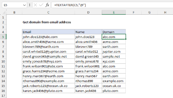
=TEXTAFTER(domain,".",-1)
Explanation
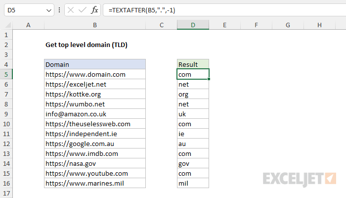
In this example, the goal is to extract the top-level domain (TLD) from a list of domains. A top-level domain is the last segment of text in a domain name, for example, ".com", ".net", or ".net". In the current version of Excel, the TEXTAFTER function is a simple way to solve this problem. In an older version of Excel, you can use a more complicated formula based on several text functions including RIGHT, FIND, LEN, and SUBSTITUTE. Both approaches are explained below.
TEXTAFTER function
The TEXTAFTER function returns the text that occurs after a given delimiter. The generic syntax for TEXTAFTER supports many options:
=TEXTAFTER(text,delimiter,[instance_num],[match_mode],[match_end], [if_not_found])
However, for this problem, we only need to provide the first three arguments:
=TEXTAFTER(text,delimiter,instance_num)
In the worksheet shown, the formula in cell D5 is:
=TEXTAFTER(B5,".",-1)
The TEXTAFTER function is configured with the following inputs:
- text - the domain in cell B5
- delimiter - a dot (".")
- instance_num - given as -1 for the last instance
With the text "https://www.domain.com" in cell B5, TEXTAFTER splits the string at the last "." and returns "com", which is the top-level domain. As the formula is copied down, the other top-level domains are returned.
For more on TEXTAFTER, see How to use the TEXTAFTER function.
Legacy Excel
Older versions of Excel do not provide the TEXTAFTER function. However, you can still extract the top-level domain (TLD)with a more complicated formula based on several text functions including RIGHT, FIND, LEN, and SUBSTITUTE:
=RIGHT(B5,LEN(B5)-FIND("*",SUBSTITUTE(B5,".","*",LEN(B5)-LEN(SUBSTITUTE(B5,".","")))))
This is an intimidating formula, complicated by the fact that the text functions in older versions of Excel are quite limited. However, it operates in a series of small steps. At the core, the formula uses the RIGHT function to extract characters starting from the right. All of the other functions in this formula just do one thing: they figure out how many characters (n) need to be extracted:
=RIGHT(B5,n) // n = ??
At a high level, the formula replaces the last dot "." in the domain with an asterisk (*) and then uses the FIND function to locate the position of the asterisk. Once the position is known, the RIGHT function is used to extract the TLD. How does the formula know to replace only the last dot? This is the clever and complicated part. The key is here:
SUBSTITUTE(B5,".","*",LEN(B5)-LEN(SUBSTITUTE(B5,".","")))
This snippet does the actual replacement of the last dot with an asterisk (*). The trick is that the SUBSTITUTE function has an optional fourth argument that specifies which "instance" of the old_text should be replaced. If no value is supplied for instance_num, SUBSTITUTE will replace all instances of old_text with new_text. However, if an instance_num is provided, SUBSTITUTE will only replace that particular instance of old_text (i.e. if 2 is provided, SUBSTITUTE will replace the second instance). Figuring out which instance to replace is the hardest part of this problem because we have no direct way to count how many dots are in a text string. Instead, we need to take a manual approach based on the LEN function:
LEN(B5)-LEN(SUBSTITUTE(B5,".",""))
Here, we calculate the total number of characters in the domain with LEN, then we subtract the total number of characters with all dots removed with the SUBSTITUTE function. For example, the value in cell B5 is "https://www.domain.com". The above expression evaluates like this:
=LEN(B5)-LEN(SUBSTITUTE(B5,".",""))
=22-20
=2
The result (2) is the number of dots in the text, which is provided to SUBSTITUTE as instance_num:
SUBSTITUTE(B5,".","*",2)
SUBSTITUTE then replaces only the second dot with "" resulting in the text "https://www.domaincom". Next, the FIND function locates the asterisk in the text:
FIND("*","https://www.domain*com") // returns 19
The result from FIND is 19, which is subtracted from the total length of the domain:
=LEN(B5)-19
=22-19
=3
The number 3 is returned to the FIND function as num_chars:
=RIGHT(B5,3) // returns "com"
And the final result returned by RIGHT is "com"