Summary
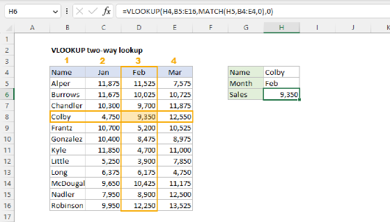
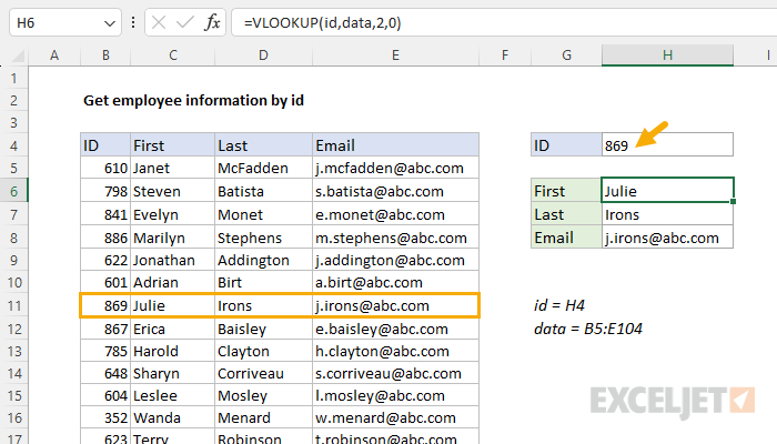
To look up employee information in a table with a unique id in the first column, you can use the VLOOKUP function. In the example shown, the formula in cell H6 is:
=VLOOKUP(id,data,2,0)
where id (H4) and data (B4:E104) are named ranges.
Note: although VLOOKUP is a simple way to solve this problem, you can also use XLOOKUP. Using XLOOKUP with a single table (the named range data) is an interesting challenge. See below for details.
Generic formula
=VLOOKUP(id,data,column,0)
Explanation
The goal is to look up and retrieve employee information in a table that contains unique id values in the first column. The VLOOKUP function is straightforward to use with data in this format, but you can easily use the XLOOKUP function as well. See below for a detailed explanation of both approaches. For convenience, id (H4) and data (B4:E104) are named ranges.
VLOOKUP function
VLOOKUP is an Excel function to get data from a table organized vertically. Lookup values must appear in the first column of the table passed into VLOOKUP. The data to retrieve is specified by column number, and the generic syntax for VLOOKUP looks like this:
=VLOOKUP(lookup_value,table_array,column_index_num,range_lookup)
The syntax looks a bit scary in this form, but it is quite simple in practice. The formulas below show how to get the first name, last name, and email address with VLOOKUP:
=VLOOKUP(id,data,2,0) // first
=VLOOKUP(id,data,3,0) // last
=VLOOKUP(id,data,4,0) // email
In these formulas, id is the named range B4 (which contains the lookup value), and data is the named range B4:E104 (the data in the table). Next, we have the column number, which is a number that indicates the column from which we want to retrieve data, where the first column is column 1 and contains lookup values. We provide 2 to retrieve the first name, 3 to retrieve the last name, and 4 to retrieve the email address. Notice that this is the only thing changing in the formulas above, every other input remains the same. Finally, we have the last value, which is zero (0). We use zero in these formulas to tell VLOOKUP to only perform an exact match. In "exact match mode" VLOOKUP will only match an id value exactly. If an id is not found, VLOOKUP will return the #N/A error. With the number 869 in cell H4, the formulas above return the results seen in the worksheet in column H:
=VLOOKUP(id,data,2,0) // returns "Julie"
=VLOOKUP(id,data,3,0) // returns "Irons"
=VLOOKUP(id,data,4,0) // returns "j.irons@abc.com"
To enter formulas like this, start with the first formula, then copy it down and change the column number as needed. The named ranges will behave like absolute references and will not change when the formula is copied to a new location.
Note: VLOOKUP will perform an approximate match by default. This is a dangerous default in this case because the data is not sorted, and there is a good chance that VLOOKUP will return an incorrect result. It is therefore important to require an exact match by using FALSE or 0 for the last argument, which is called "range_lookup". More information here.
XLOOKUP function
Another way to solve this problem is with XLOOKUP, a modern upgrade to the VLOOKUP function. This minimal syntax for XLOOKUP looks like this:
=XLOOKUP(lookup_value,lookup_array,return_array)
Unlike VLOOKUP, we don't give XLOOKUP the entire table. Instead, we provide separate ranges for lookup_array and return_array. The formulas to look up the first name, last name, and email address with XLOOKUP look like this:
=XLOOKUP(id,B5:B104,C5:C104) // first
=XLOOKUP(id,B5:B104,D5:D104) // last
=XLOOKUP(id,B5:B104,E5:E104) // email
Notice the only value changing is the range provided for return_array, which varies according the to information we want to retrieve. We use C5:C104 for the first name, D5:D104 for the first name, and E5:E104 for the email address. The value for lookup_value is the named range id (H4). See below for information on how to adapt this formula to use the existing named range data (B4:E104).
Note: Normally, I would use absolute references to make the formulas easier to copy, but I have left these ranges relative to make them a bit easier to read.
XLOOKUP with a named range
If we had named ranges for ids, first, last, and email defined, we could use them in XLOOKUP like this:
=XLOOKUP(id,ids,first) // first
=XLOOKUP(id,ids,last) // last
=XLOOKUP(id,ids,email) // email
Similarly, if data was a proper Excel Table, we could use structured references like so:
=XLOOKUP(id,data[Id],data[First]) // first
=XLOOKUP(id,data[Id],data[Last]) // last
=XLOOKUP(id,data[Id],data[Email]) // email
Both of these options above would work well with XLOOKUP. However, in the example shown, we only have the named range data (B5:E104). Is there a way to use the entire table directly with XLOOKUP? Yes. It's a little tricky, but we can use the CHOOSECOLS function.
XLOOKUP with CHOOSECOLS
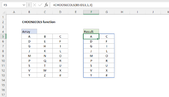
One way to use XLOOKUP with the named range data is to use the CHOOSECOLS function like this:
=XLOOKUP(id,CHOOSECOLS(data,1),CHOOSECOLS(data,2)) // first
=XLOOKUP(id,CHOOSECOLS(data,1),CHOOSECOLS(data,3)) // last
=XLOOKUP(id,CHOOSECOLS(data,1),CHOOSECOLS(data,4)) // email
The CHOOSECOLS function returns one or more columns from a range by numeric index. In the formulas above, we are using CHOOSECOLS to get the first column (1) for the lookup_array in all formulas. Then, for result_array, we vary the number as needed to get to provide the correct range for first name (2), last name (3), and email address (4).
Note: Excel purists will point out that we could also use the INDEX function to retrieve columns for XLOOKUP. Yes, absolutely.
XLOOKUP with DROP and TAKE
Yet another way to solve this problem is to use the TAKE function with the DROP function with the entire named range data:
=XLOOKUP(id,TAKE(data,,1),DROP(data,,1))
This formula will return all first, last, and email all in one step and the result will spill into the worksheet in three cells horizontally. To get all three values in a vertical array, you can wrap the above formula in the TRANSPOSE function:
=TRANSPOSE(XLOOKUP(id,TAKE(data,,1),DROP(data,,1)))
TRANSPOSE simply flips the orientation of the array returned by XLOOKUP.