Summary
To retrieve the cell value at a specific row and column number, you can use the ADDRESS function together with the INDIRECT function. In the example shown, the formula in G6 is:
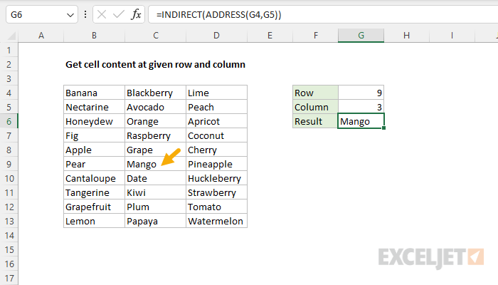
=INDIRECT(ADDRESS(G4,G5))
The result is "Mango", the value in cell C9, at row 9 and column 3 of the worksheet. Although this is one way to get the value of a cell at a known location, it is not an optimal approach. Read more below.
Generic formula
=INDIRECT(ADDRESS(row,col))
Explanation
The goal is to retrieve the value of a cell at a given row and column location, which are entered in cells G5 and G4, respectively. There are several ways to go about this, depending on your needs. See below for options.
ADDRESS and INDIRECT
In the example worksheet, the ADDRESS function is combined with the INDIRECT function to solve this problem with the following formula:
=INDIRECT(ADDRESS(G4,G5))
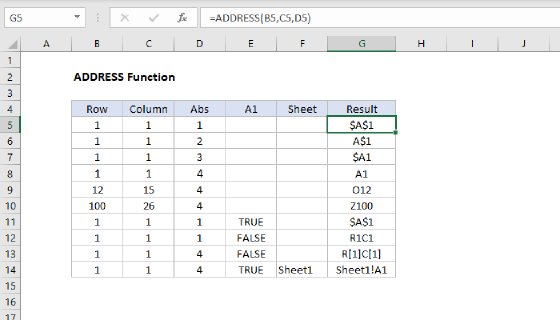
The ADDRESS function returns the address for a cell based on a given row and column number like this:
=ADDRESS(1,1) // returns $A$1
=ADDRESS(1,2) // returns $B$1
=ADDRESS(2,1) // returns $A$2
=ADDRESS(2,2) // returns $B$2
Note: ADDRESS can return references in different formats, see here for details.
In the example shown, the ADDRESS function returns the value "$C$9" inside INDIRECT:
=INDIRECT(ADDRESS(9,3))
=INDIRECT("$C$9")
The INDIRECT function converts a text value into a valid reference. INDIRECT converts the text "$C$9" into the cell reference $C$9 and returns "Mango" as the final result:
=INDIRECT("$C$9")
=$C$9
="Mango"
While this formula works, there is a better way to retrieve the cell value at a known location in Excel.
Note: INDIRECT is a volatile function and can cause performance problems in more complicated worksheets.
INDEX function
The INDEX function is well-known in Excel because it is part of INDEX and MATCH, a common way to perform lookup operations in Excel. But INDEX can also be used by itself to retrieve values at known coordinates. To solve this problem, we can give the INDEX function a range that begins at A1, and includes the cells that need to be referenced like this:
=INDEX(A1:E100,9,3) // returns "Mango"
As before, the result is "Mango" and this is a much better example of how to retrieve a value in Excel. Replacing the hardcoded row and column numbers above with worksheet references we have:
=INDEX(A1:E100,G4,G5)
This formula returns the same result seen in the screenshot. If row or column numbers change, the INDEX function returns a new result. Note that the size of the range we give INDEX is arbitrary, but it must start at A1 and include the data you wish to reference.
Note: In most cases, INDEX is not used by itself in a formula because the row and column numbers are often unknown. Instead, INDEX is combined with the MATCH function, which calculates the required row and column positions. Read more here.