FILTER with multiple OR criteria

To extract data with multiple OR conditions, you can use the FILTER function together with the MATCH function. In the example shown, the formula in F9 is:

=FILTER(B5:D16,
ISNUMBER(MATCH(items,F5:F6,0))*
ISNUMBER(MATCH(colors,G5:G6,0))*
ISNUMBER(MATCH(cities,H5:H6,0)))

where items (B3:B16), colors (C3:C16), and cities (D3:D16) are named ranges.

This formula returns data where item is (tshirts OR hoodie) AND color is (red OR blue) AND city is (denver OR seattle).

Explanation

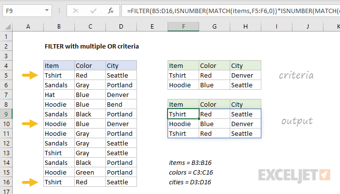
In this example, criteria are entered in the range F5:H6. The logic of the formula is:

item is (tshirt OR hoodie) AND color is (red OR blue) AND city is (denver OR seattle)

The filtering logic of this formula (the include argument) is applied with the ISNUMBER and MATCH functions, together with boolean logic applied in an array operation.

MATCH is configured "backwards", with lookup_values coming from the data, and criteria used for the lookup_array. For example, the first condition is that items must be either a Tshirt or Hoodie. To apply this condition, MATCH is set up like this:

MATCH(items,F5:F6,0) // check for tshirt or hoodie

Because there are 12 values in the data, the result is an array with 12 values like this:

{1;#N/A;#N/A;2;#N/A;2;2;#N/A;1;#N/A;2;1}

This array contains either #N/A errors (no match) or numbers (match). Notice numbers correspond to items that are either Tshirt or Hoodie. To convert this array into TRUE and FALSE values, the MATCH function is wrapped in the ISNUMBER function:

ISNUMBER(MATCH(items,F5:F6,0))

which yields an array like this:

{TRUE;FALSE;FALSE;TRUE;FALSE;TRUE;TRUE;FALSE;TRUE;FALSE;TRUE;TRUE}

In this array, the TRUE values correspond to tshirt or hoodie.

The full formula contains three expressions like the above used for the include argument of the FILTER function:

ISNUMBER(MATCH(items,F5:F6,0))* // tshirt or hoodie
ISNUMBER(MATCH(colors,G5:G6,0))* // red or blue
ISNUMBER(MATCH(cities,H5:H6,0))) // denver or seattle

After MATCH and ISNUMBER are evaluated, we have three arrays containing TRUE and FALSE values. The math operation of multiplying these arrays together coerces the TRUE and FALSE values to 1s and 0s, so we can visualize the arrays at this point like this:

{1;0;0;1;0;1;1;0;1;0;1;1}*
{1;0;1;1;0;1;0;0;0;0;0;1}*
{1;0;1;0;0;1;0;1;1;0;0;1}

The result, following the rules of boolean arithmetic, is a single array:

{1;0;0;0;0;1;0;0;0;0;0;1}

which becomes the include argument in the FILTER function:

=FILTER(B5:D16,{1;0;0;0;0;1;0;0;0;0;0;1})

The final result is the three rows of data shown in F9:H11

With hard-coded values

Although the formula in the example uses criteria entered directly on the worksheet, criteria can be hard-coded as array constants instead like this:

=FILTER(B5:D16,
ISNUMBER(MATCH(items,{"Tshirt";"Hoodie"},0))*
ISNUMBER(MATCH(colors,{"Red";"Blue"},0))*
ISNUMBER(MATCH(cities,{"Denver";"Seattle"},0)))