Explanation
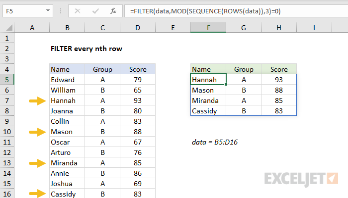
The FILTER function is designed to filter and extract information based on logical criteria. In this example, the goal is to extract every 3rd record from the data shown, but there is no row number information in the data.
Working from the inside out, the first step is to generate a set of row numbers. This is done with the SEQUENCE function like this:
SEQUENCE(ROWS(data))
The ROW function returns the count of rows in the named range data. Using the count of rows, SEQUENCE returns an array of 12 numbers in sequence:
{1;2;3;4;5;6;7;8;9;10;11;12}
This array is returned directly to the MOD function as the number argument, with the number 3 hardcoded as the divisor. MOD is set up to test if row numbers are divisible by 3 with a remainder of zero
MOD(SEQUENCE(ROWS(data)),3)=0 // divisible by 3?
The result from MOD is an array or TRUE and FALSE values like this:
{FALSE;FALSE;TRUE;FALSE;FALSE;TRUE;FALSE;FALSE;TRUE;FALSE;FALSE;TRUE}
Note TRUE values correspond with every 3rd row in the data. This array is delivered directly to the FILTER function as the include argument. FILTER returns every 3rd row in data as a final result.


