Explanation
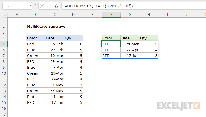
This formula relies on the FILTER function to retrieve data based on a logical test. The array argument is provided as B5:D15, which contains all of the data without headers. The include argument is an expression based on the EXACT function:
EXACT(B5:B15,"RED")
The EXACT function compares two text strings in a case-sensitive manner. If the two strings are exactly the same, EXACT returns TRUE. If the two strings are not exactly the same, EXACT returns FALSE. Since we are giving EXACT a range with 11 values as the first argument, and the string "RED" as the second, EXACT returns an array with 11 results like this:
{FALSE;FALSE;FALSE;TRUE;FALSE;FALSE;TRUE;FALSE;FALSE;FALSE;TRUE}
Notice the position of TRUE values in this array corresponds to the rows where the color is "RED".
This array returned directly to the FILTER function as the include argument. FILTER uses the array to filter the range B5:D15, and returns the three rows where the color is "RED". Rows where the color is "Red" are not included.
Partial match
To run an exact match with FILTER based on a partial match, see the example explained here.
Dynamic Array Formulas are available in Office 365 only.


