Summary
To filter data to include data based on dates, you can use the FILTER function with one or more of Excel's date functions. In the example shown, we are filtering by month with the MONTH function. The formula in E5 is:
=FILTER(B5:C16,MONTH(B5:B16)=11,"No data")
The result returned by FILTER includes only rows where the date falls in November. See below for other filter-by-date examples.
Generic formula
=FILTER(range,MONTH(dates)=n,"No data")
Explanation
This example shows how to filter dates using Excel's FILTER function. Several common date-based filtering patterns are shown below, including filtering by month, filtering by a specific date, and filtering by month and year.
Filter by month
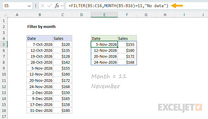
In the worksheet below, the goal is to filter the data to include only rows where the date falls in November. The formula in cell E5 is:
=FILTER(B5:C16,MONTH(B5:B16)=11,"No data")
Note that the month is hardcoded as the number 11. The result returned by FILTER includes only rows where the date falls in November:

This formula relies on the FILTER function to retrieve data based on a logical test created with the MONTH function. The array argument is B5:C16, which contains the full set of data without headers. The include argument is constructed with the MONTH function:
MONTH(B5:B16)=11
Here, MONTH receives the range B5:B16. Since the range contains 12 cells, MONTH returns an array with 12 results representing each date's month number:
{10;10;10;10;11;11;11;11;12;12;12;12}
Each result is then compared to 11 (November), and this operation creates an array of 12 TRUE and FALSE values, which is delivered to the FILTER function as the include argument:
{FALSE;FALSE;FALSE;FALSE;TRUE;TRUE;TRUE;TRUE;FALSE;FALSE;FALSE;FALSE}
FILTER uses this array to select specific rows. Only rows where the result is TRUE make it into the final output. The if_empty argument is set to "No data" in case no matching data is found.
Filter by specific date
To filter by a specific date, use the DATE function to construct the date value for comparison. You can see how this works in the worksheet below, where the formula in E5 is:
=FILTER(B5:C16,B5:B16=DATE(2026,11,24),"No data")
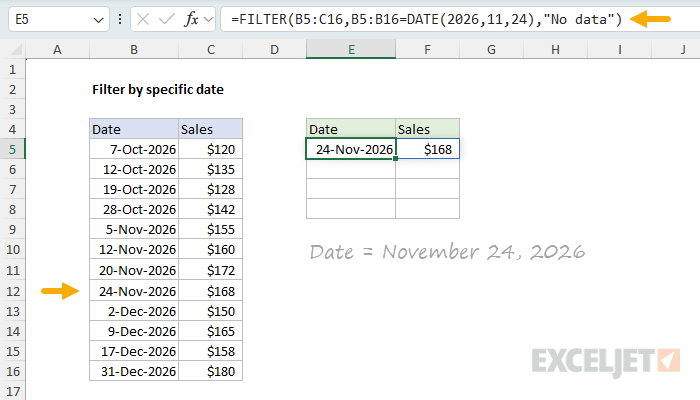
The DATE function creates a proper Excel date from the year (2026), month (11), and day (24). This is compared against each date in the range B5:B16. Only the row matching November 24, 2026 is returned.
Filter by month and year
To filter by both month and year, you can construct a formula using boolean logic that combines the YEAR function and MONTH function:
=FILTER(B5:C16,(YEAR(B5:B16)=2026)*(MONTH(B5:B16)=12),"No results")
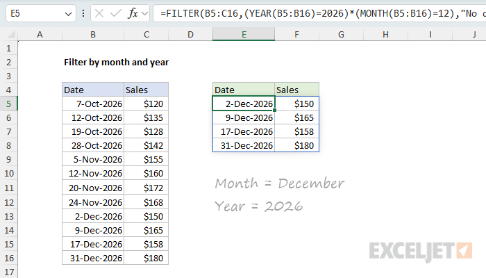
The multiplication operator (*) acts as an AND condition—both the year must equal 2026 and the month must equal 12 (December) for a row to be included. This returns all four December 2026 dates from the source data.
Although the values for month and year are hardcoded in this example (the year is 2026 and the month is 12), these values can easily be replaced with cell references to make the formula more flexible.
Summary
The FILTER function can extract data by date in different ways using Excel's date functions:
- Use MONTH, YEAR, DAY, or WEEKDAY to extract date components
- Compare extracted values to target values to create a Boolean array
- Combine multiple criteria with multiplication (AND logic)
- Use cell references instead of hardcoded values for flexibility
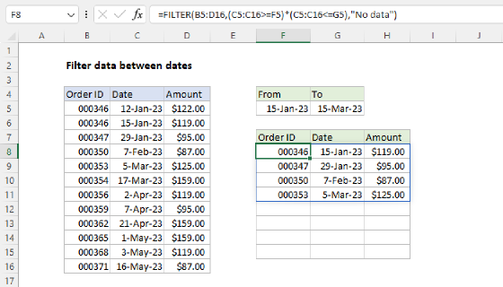
For filtering between two dates, see Filter data between dates.