Summary
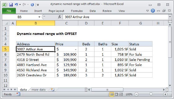
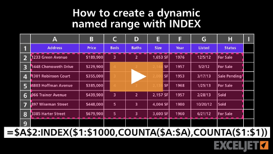
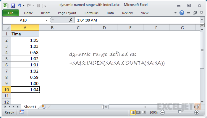
One way to create a dynamic named range in Excel is to use the INDEX function. In the example shown, the named range "data" is defined by the following formula:
=$A$2:INDEX($A:$A,COUNTA($A:$A))
This formula resolves to the range $A$2:$A$10.
Note: this formula is meant to define a named range that can be used in other formulas. This range will be dynamic and expand and shrink with the data. An alternative to a formula-based dynamic named range is to use an Excel Table. If you are using Excel 365 another option is to use the TRIMRANGE function, which is designed to create dynamic ranges.
Generic formula
=$A$1:INDEX($A:$A,lastrow)
Explanation
This page shows an example of a dynamic named range created with the INDEX function together with the COUNTA function. Dynamic named ranges automatically expand and contract when data is added or removed. They are an alternative to using an Excel Table, which also resizes as data is added or removed.
The INDEX function returns the value at a given position in a range or array. You can use INDEX to retrieve individual values or entire rows and columns in a range. What makes INDEX especially useful for dynamic named ranges is that it actually returns a reference. This means you can use INDEX to construct a mixed reference like $A$1:A100.
In the example shown, the named range "data" is defined by the following formula:
=$A$2:INDEX($A:$A,COUNTA($A:$A))
which resolves to the range $A$2:$A$10.
How this formula works
Note first that this formula is composed of two parts that sit on either side of the range operator (:). On the left, we have the starting reference for the range, hard coded as:
$A$2
On the right is the ending reference for the range, created with INDEX like this:
INDEX($A:$A,COUNTA($A:$A))
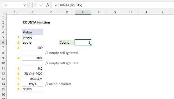
Here, we feed INDEX all of column A for the array, then use the COUNTA function to figure out the "last row" in the range. COUNTA works well here because there are 10 values in column A, including a header row. COUNTA therefore returns 10, which goes directly into INDEX as the row number. INDEX then returns a reference to $A$10, the last used row in the range:
INDEX($A:$A,10) // resolves to $A$10
So, the final result of the formula is this range:
$A$2:$A$10
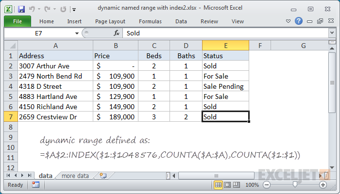
A two-dimensional range
The above example works for a one-dimensional range. To create a two-dimensional dynamic range where the number of columns is also dynamic, you can use the same approach, expanded like this:
=$A$2:INDEX($1:$1048576,COUNTA($A:$A),COUNTA($1:$1))
As before, COUNTA is used to figure out the "lastrow", and we use COUNTA again to get the "lastcolumn". These are supplied to INDEX as row_num and column_num respectively.
However, for the array, we supply the full worksheet, entered as all 1048576 rows, which allows INDEX to return a reference in a 2D space.
Determining the last row
There are several ways to determine the last row (last relative position) in a set of data, depending on the structure and content of the data in the worksheet: