Last row in mixed data with blanks

To get the last relative position (i.e. last row, last column) for mixed data that may contain empty cells, you can use the MATCH function as described below. In the example shown, the formula in E5 is:

{=MATCH(2,1/(B4:B10<>""))}

Note: this is an array formula and must be entered with Control+Shift+Enter.

Explanation

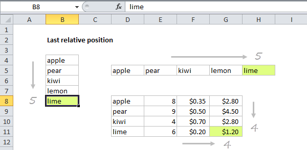
When constructing more advanced formulas, it's often necessary to figure out the last location of data in a list. Depending on the data, this could be the last row with data, the last column with data, or the intersection of both. We want the last *relative position* inside a given range not the row number on the worksheet:

Illustration of last relative position (last row, last column)

This formula uses the MATCH function configured to find the position of the last non-empty cell in a range. Working from the inside out, the lookup array inside MATCH is constructed like this:

=1/(B4:B10<>""))
=1/{TRUE;FALSE;TRUE;FALSE;TRUE;TRUE;FALSE}
={1;#DIV/0!;1;#DIV/0!;1;1;#DIV/0!}

Note: all values in the array are either 1 or the #DIV/0! error.

MATCH is then set to match the value 2 in "approximate match mode", by omitting the 3rd argument is omitted.

Because the lookup value of 2 will never be found, MATCH will always find the last 1 in the lookup array, which corresponds to the last non-empty cell.

This approach will work with any kind of data, including numbers, text, dates, etc. It also works with null text strings that are returned by formulas like this:

=IF(A1<100,"")

Dynamic range

You can use this formula to create a dynamic range with other functions like INDEX and OFFSET. See the links below for examples:

Inspiration for this article came from Mike Girvin's excellent book Control + Shift + Enter, where Mike does a great job explaining the concept of "last relative position".