Summary
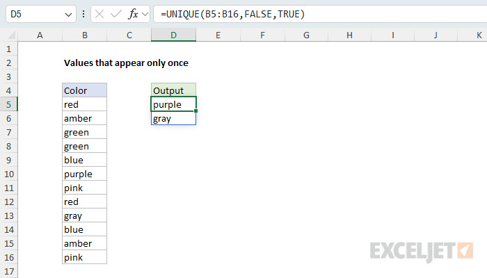
To extract a list of values that appear only once in a set of data, you can use the UNIQUE function with the exactly_once argument set to TRUE. In the example shown, the formula in D5 is:
=UNIQUE(B5:B16,FALSE,TRUE)
The result is the 2 values in B5:B16 that appear exactly one time, "purple" and "gray". Every other color in the list appears at least twice, so it is excluded.
This is a different problem from extracting unique values. A list of unique values includes every value in the data once, no matter how many times it appears. This page is about values that occur exactly one time in the source data. For the general case, see Unique values and the UNIQUE function.
Generic formula
=UNIQUE(data,FALSE,TRUE)
Explanation
In this example, the goal is to list the values in B5:B16 that appear only once. The data contains 12 colors. Most of them appear twice, but "purple" and "gray" each appear just once, and these are the values we want to extract.
Before dynamic arrays, this was a surprisingly awkward problem in Excel. In the current version of Excel, the UNIQUE function solves it directly with an optional argument, as explained below. The page also shows how to sort and count the results, how to flip the logic to find values that appear more than once, and some options for solving the problem in Legacy Excel.
Table of contents
- Unique values vs. values that appear once
- The exactly_once argument
- Sort the results
- Count values that appear only once
- Values that appear more than once
- Dynamic source range
- Legacy Excel
- Summary
Unique values vs. values that appear once
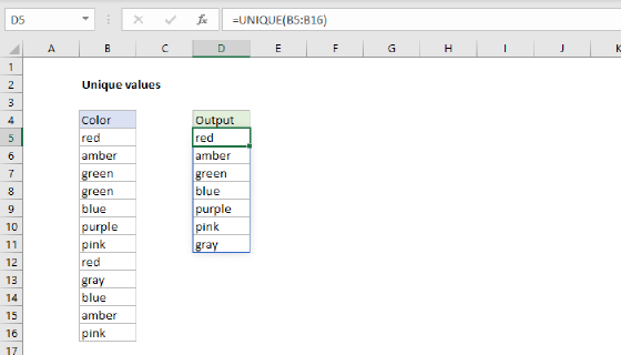
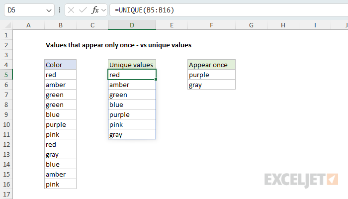
One thing that confuses people is the difference between "unique values" and "values that appear only once", because both phrases get used loosely. In Excel, the UNIQUE function uses "unique" to mean a distinct list: every value in the data, listed one time. With default settings, UNIQUE returns this kind of list:
=UNIQUE(B5:B16)
With the data in the example, this formula returns 7 values:
{"red";"amber";"green";"blue";"purple";"pink";"gray"}
Notice that "red" appears twice in the data but only once in the result. That is the whole point of a unique list. The question on this page is narrower: which values appear exactly one time in the source data? For the same data, the answer is 2 values:
{"purple";"gray"}
Both results come from the UNIQUE function. The difference is the third argument, exactly_once. Values that appear only once are sometimes called "distinct values", but that term gets used both ways too, so this page sticks with "values that appear only once".
The exactly_once argument
The UNIQUE function takes three arguments: array, by_col, and exactly_once. The last two are optional:
- array is the range or array to evaluate. In this example, it is B5:B16.
- by_col controls whether UNIQUE compares values by row (FALSE, the default) or by column (TRUE). The data in this example is in a single column, so we use FALSE.
- exactly_once controls what counts as unique. With FALSE (the default), UNIQUE returns every distinct value. With TRUE, UNIQUE returns only values that appear exactly one time.
In the example shown, the formula in D5 sets exactly_once to TRUE:
=UNIQUE(B5:B16,FALSE,TRUE)
UNIQUE evaluates the 12 values in B5:B16 and returns the 2 values that appear once, "purple" and "gray". The result spills into D5:D6. If a value in B5:B16 changes, the result updates automatically. For example, if the second "pink" in B16 is changed to "brown", both "pink" and "brown" will appear once, and UNIQUE will return 4 values.
Because by_col defaults to FALSE, you can leave it out and keep the comma as a placeholder:
=UNIQUE(B5:B16,,TRUE)
You can also use 1 and 0 instead of TRUE and FALSE:
=UNIQUE(B5:B16,0,1)
All three formulas return the same result.
Sort the results
UNIQUE returns values in the order they first appear in the data. To sort the results alphabetically, wrap the formula in the SORT function:
=SORT(UNIQUE(B5:B16,,TRUE)) // returns {"gray";"purple"}
SORT sorts in ascending order by default. To sort in descending order, provide -1 for the sort_order argument:
=SORT(UNIQUE(B5:B16,,TRUE),,-1) // returns {"purple";"gray"}
Count values that appear only once
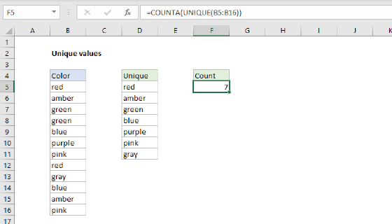
To count the values that appear only once instead of listing them, wrap UNIQUE in the ROWS function:
=ROWS(UNIQUE(B5:B16,,TRUE)) // returns 2
One caveat: if no values appear exactly once, UNIQUE returns a #CALC! error, and ROWS returns the same error. To return zero instead, wrap the formula in the IFERROR function:
=IFERROR(ROWS(UNIQUE(B5:B16,,TRUE)),0)
To count unique values in the general sense, see Count unique values.
Values that appear more than once
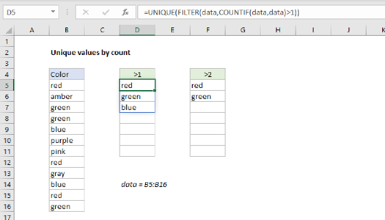
The flip side of this problem is to list values that appear more than once, in other words, the duplicates. UNIQUE can't do this on its own, because exactly_once only has two settings. Instead, use the FILTER function with COUNTIF to keep values that appear more than once, then use UNIQUE to remove the repeats:
=UNIQUE(FILTER(B5:B16,COUNTIF(B5:B16,B5:B16)>1))
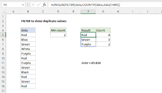
With the data in the example, this formula returns 5 values: "red", "amber", "green", "blue", and "pink". The formula is explained in detail on the Unique values by count page. To list every duplicate row instead of a distinct list of duplicates, see Filter to show duplicate values.
Dynamic source range
UNIQUE won't automatically change the source range if data is added or deleted. To give UNIQUE a dynamic range that will automatically resize as needed, you can use an Excel Table, or create a dynamic named range with a formula. In Excel 365, you can also use the TRIMRANGE function or the dot operator.
Legacy Excel
UNIQUE is available in Excel 2021+ and Excel 365. In older versions of Excel, the simplest approach is a helper column based on the COUNTIF function (see also Alternatives to dynamic array functions). With the data in B5:B16, the formula in a helper column, copied down, looks like this:
=COUNTIF($B$5:$B$16,B5)=1
COUNTIF counts how many times the value in B5 appears in the full range. The range is locked with an absolute reference so it doesn't change as the formula is copied down, while B5 is relative and changes on each row. When the count is 1, the formula returns TRUE; otherwise it returns FALSE. Once the helper column is in place, you can filter the data on TRUE. The same test can also be used as a conditional formatting rule to highlight values that appear once directly in the data.
To count values that occur just once in an older version of Excel, you can use a formula based on the COUNTIF function and the SUMPRODUCT function like this:
=SUMPRODUCT(--(COUNTIF(B5:B16,B5:B16)=1)) // returns 2
Here, COUNTIF returns a count for every value in the data, the comparison =1 converts the counts to TRUE and FALSE, the double negative (--) converts TRUE and FALSE to 1 and 0, and SUMPRODUCT sums the result. This is the same test used in the helper column above, applied to the whole range at once.
Summary
UNIQUE with exactly_once set to TRUE is the modern answer to a question that used to be hard in Excel: which values in a list appear only once?
- "Unique values" and "values that appear only once" are different questions. UNIQUE with default settings lists every value once; UNIQUE with exactly_once set to TRUE lists only values that occur one time. For the general case, see Unique values.
- Wrap UNIQUE in SORT to sort the results and in ROWS to count them. Use IFERROR to handle the #CALC! error that occurs when no values appear once.
- To find values that appear more than once, combine UNIQUE with FILTER and COUNTIF.
- In Legacy Excel, use
COUNTIF(data,A1)=1in a helper column to flag values that appear once, or SUMPRODUCT with COUNTIF to count them.