Summary
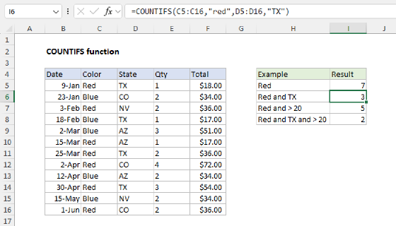
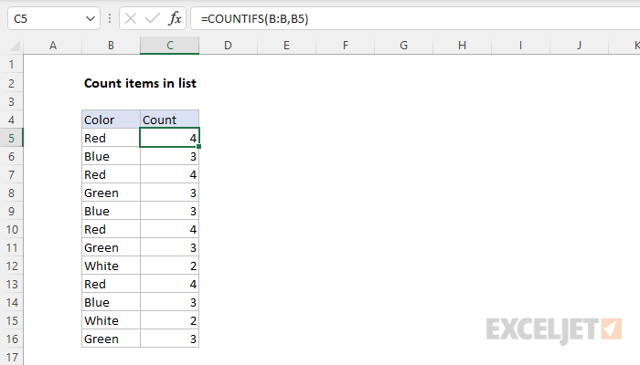
To create a count of the values that appear in a list or table, you can use the COUNTIFS function. In the example shown, the formula in C5 is:
=COUNTIFS(B:B,B5)
As the formula is copied down, it returns a count of each color in column B. This formula uses the full column reference B:B for convenience. You can also use an absolute reference like $B$5:$B$16. An Excel Table would also be a good option.
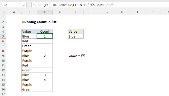
See also: Running count of occurrence in list, and Summary count with COUNTIFS
Generic formula
=COUNTIFS(A:A,A1)
Explanation
In this example, the goal is to create a count of each color in column B. The simplest way to solve this problem is with the COUNTIFS function.
COUNTIFS function
The COUNTIFS function returns the count of cells that meet one or more criteria. COUNTIFS can be used with criteria based on dates, numbers, text, and other conditions. COUNTIFS supports logical operators (>,<,<>,=) and wildcards (*,?) for partial matching. To configure COUNTIFS, conditions are supplied in range/criteria pairs — each pair contains one range and the associated criteria for that range:
=COUNTIFS(range1,criteria1,range2,criteria2,etc.)
In this example, we want to count each value in column B, starting with cell B5. To do this, we can use a formula like this in cell C5:
=COUNTIFS(B:B,B5) // returns 4
The result in cell C5 is 4, since "Red" appears 4 times in column B. As the formula is copied down, it returns a count for each value in B5:B16. Note this formula uses the full column reference B:B for convenience. You can also use an absolute reference like this:
=COUNTIFS($B$5:$B$16,B5)
As an alternative, you could use an Excel Table to hold the data, and then use a structured reference.
With two criteria
In the workbook below, we have Color and Price. By adding a second range/criteria pair to COUNTIFS, we can count the combination of Color and Price like this:
=COUNTIFS(B:B,B5,C:C,C5)

Because both range/criteria pairs appear in the same COUNTIFS function, they link the values in column B with those in column C, and COUNTIFS generates a count of each Color and Price combination that appears in the table. Notice these counts differ from the original example above because some of the same colors have different prices.