Summary
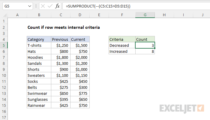
To count rows in a table that meet internal, calculated criteria, without using a helper column, you can use the SUMPRODUCT function. In the example shown, the formula in cell G5 is:
=SUMPRODUCT(--(C5:C15>D5:D15))
The result is 3, since there are three rows where Previous sales are greater than Current sales.
Generic formula
=SUMPRODUCT(--(logical_expression))
Explanation
In this example the goal is to count products (rows) where sales have increased and sales have decreased, where previous sales are in column C (Previous) and current sales are in column D (Current). In this case, we can't use COUNTIFS directly, because COUNTIFS is a range-based function and it won't accept a calculation for a range argument. One option is to add a helper column that subtracts Previous sales from Current sales and use COUNTIF to count results less than or greater than zero. But what if we don't want to (or can't) add a helper column? In that case, we can use the SUMPRODUCT function with Boolean logic.
SUMPRODUCT function
The SUMPRODUCT function is designed to work with arrays. It multiplies corresponding elements in two or more arrays and sums the resulting products. One of SUMPRODUCT's special features is that it can handle "array operations" natively, without requiring Control + Shift + Enter. This allows us to perform a comparison between current and previous sales directly in array1. To count rows where sales have decreased, we simply compare the values in column C to the values in column D using a logical expression like this:
C5:C15>D5:D15
The result is an array of TRUE FALSE values like this:
{FALSE;TRUE;FALSE;TRUE;FALSE;FALSE;FALSE;FALSE;TRUE;FALSE;FALSE}
To coerce the TRUE and FALSE values to 1s and 0s, we use a double negative (--):
--(C5:C15>D5:D15)
This operation creates an array like this:
{0;1;0;1;0;0;0;0;1;0;0}
Notice the 1s correspond to TRUE values in the previous array. The numeric array is returned to SUMPRODUCT as array1:
=SUMPRODUCT({0;1;0;1;0;0;0;0;1;0;0}) // returns 3
Since there is only one array to process, SUMPRODUCT simply returns a sum. The result is 3 since there are three rows where the value in column C is greater than the value in column D.
Sales increased
To count rows where sales have increased, we can simply reverse the logic. The formula in G6 is:
=SUMPRODUCT(--(C5:C15<D5:D15))
The result is 8, since there are 8 rows where Previous sales are less than Current sales.