Summary
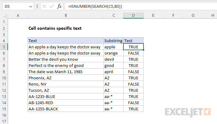
To check if a cell contains specific text (i.e. a substring), you can use the SEARCH function together with the ISNUMBER function. In the example shown, the formula in D5 is:
=ISNUMBER(SEARCH(C5,B5))
This formula returns TRUE if the substring in cell C5 is found in the text from cell B5. Otherwise, it returns FALSE. Note the SEARCH function is not case-sensitive. See below for a case-sensitive formula.
Generic formula
=ISNUMBER(SEARCH(substring,A1))
Explanation
In this example, the goal is to test a value in a cell to see if it contains a specific substring. Excel contains two functions designed to check the occurrence of one text string inside another: the SEARCH function and the FIND function. The difference is that the SEARCH function supports wildcards but is not case-sensitive, while the FIND function is case-sensitive but does not support wildcards. Both functions return the position of the substring in the text as a number when it is found and a #VALUE! error when the substring is not found. However, it is not obvious how to get a TRUE or FALSE result when the goal is simply to test for the existence of the substring. The standard approach is to wrap these functions in the ISNUMBER function to force a TRUE or FALSE result. ISNUMBER will return TRUE for a numeric result (a match) and FALSE when the result is #VALUE! (no-match).
Excel 365 now supports regular expressions (regex), a powerful tool for pattern-matching. The REGEXTEST function offers a direct way to test for specific text with a TRUE or FALSE result. Because REGEXTEST uses regex, it can be configured to use precise patterns for advanced use cases. See below for basic examples.
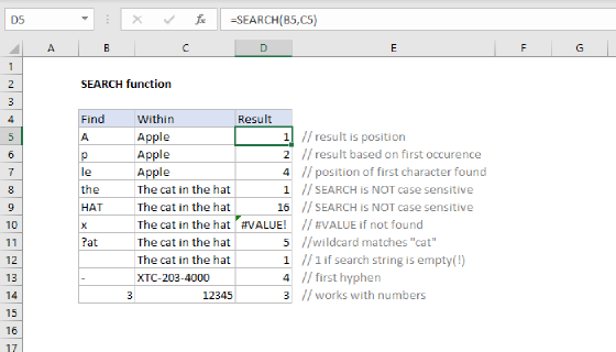
SEARCH function (not case-sensitive)
The SEARCH function is designed to look inside a text string for a specific substring. If SEARCH finds the substring, it returns the position of the substring in the text as a number. If the substring is not found, SEARCH returns a #VALUE error. For example:
=SEARCH("p","apple") // returns 2
=SEARCH("z","apple") // returns #VALUE!
To force a TRUE or FALSE result, we use the ISNUMBER function. ISNUMBER returns TRUE for numeric values and FALSE for anything else. So, if SEARCH finds the substring, it returns the position as a number, and ISNUMBER returns TRUE:
=ISNUMBER(SEARCH("p","apple")) // returns TRUE
=ISNUMBER(SEARCH("z","apple")) // returns FALSE
If SEARCH doesn't find the substring, it returns an error, which causes the ISNUMBER to return FALSE.
Wildcards
Although SEARCH is not case-sensitive, it does support wildcards (*?~). For example, the question mark (?) wildcard matches any one character. The formula below looks for a 3-character substring beginning with "x" and ending in "y":
=ISNUMBER(SEARCH("x?z","xyz")) // TRUE
=ISNUMBER(SEARCH("x?z","xbz")) // TRUE
=ISNUMBER(SEARCH("x?z","xyy")) // FALSE
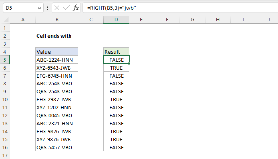
The asterisk (*) wildcard matches zero or more characters. This wildcard is not as useful in the SEARCH function because SEARCH already looks for a substring. For example, it might seem like the following formula will test for a value that ends with "z":
=ISNUMBER(SEARCH("*z",text))
However, because SEARCH automatically looks for a substring, the following formulas all return 1 as a result, even though the text in the first formula is the only text that ends with "z":
=SEARCH("*z","XYZ") // returns 1
=SEARCH("*z","XYZXY") // returns 1
=SEARCH("*z","XYZXY123") // returns 1
=SEARCH("x*z","XYZXY123") // returns 1
This means the asterisk () is not a reliable way to test for "ends with". However, you can use the asterisk () wildcard like this:
=SEARCH("x*2*b","AAAXYZ123ABCZZZ") // returns 4
=SEARCH("x*2*b","NXYZ12563JKLB") // returns 2
Here we are looking for "x", "2", and "b" in that order, with any number of characters in between. Finally, you can use the tilde (~) as an escape character to indicate that the next character is a literal like this:
=SEARCH("~*","apple*") // returns 6
=SEARCH("~?","apple?") // returns 6
=SEARCH("~~","apple~") // returns 6
The above formulas use SEARCH to find a literal asterisk (*), question mark (?), and tilde (~) in that order.
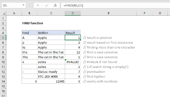
FIND function (case-sensitive)
Like the SEARCH function, the FIND function returns the position of a substring in text as a number, and an error if the substring is not found. However, unlike the SEARCH function, the FIND function respects case:
=FIND("A","Apple") // returns 1
=FIND("A","apple") // returns #VALUE!
To make a case-sensitive version of the formula, just replace the SEARCH function with the FIND function in the formula above:
=ISNUMBER(FIND(substring,A1))
The result is a case-sensitive search:
=ISNUMBER(FIND("A","Apple")) // returns TRUE
=ISNUMBER(FIND("A","apple")) // returns FALSE
REGEXTEST function (very powerful)
The REGEXTEST function tests for text defined by a given pattern. Regex patterns are very flexible and can be configured to match numbers, email addresses, dates, and other values that have an identifiable pattern. The generic syntax for REGEXTEST looks like this:
=REGEXTEST(text,pattern)
The text is the text to search within, and the pattern is the text to search for, which can be a hardcoded text string or a combination of special characters used to define regex patterns. The result from REGEXTEST is TRUE or FALSE, so there is no need for ISNUMBER:
=REGEXTEST("apple","a") // returns TRUE
=REGEXTEST("apple","z") // returns FALSE
Note that REGEXTEST is case-sensitive by default:
=REGEXTEST("apple","A") // returns FALSE
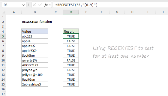
The power of REGEXTEST comes from its ability to use regex patterns. Here are a few simple examples that check text in cell A1 for various things:
=REGEXTEST(A1,"[0-9]") // test for a number
=REGEXTEST(A1,"[A-Z]") // test for an uppercase character
=REGEXTEST(A1,"\d{3}") // test for a 3-digit number
=REGEXTEST(A1,"[A-Z]{3}") // test for 3 uppercase characters together
Here are the examples above applied to a text string:
=REGEXTEST("apple9","[0-9]") // returns TRUE
=REGEXTEST("appLe","[A-Z]") // returns TRUE
=REGEXTEST("apple123","\d{3}") // returns TRUE
=REGEXTEST("appleABC","[A-Z]{3}") // // returns TRUE
For an overview of regex in Excel, see Regular Expressions in Excel.
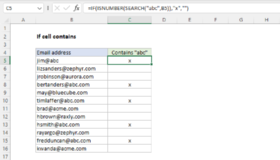
If cell contains
To return a custom result when a cell contains specific text, you can wrap the formulas above inside the IF function like this:
=IF(ISNUMBER(SEARCH(substring,A1)),"Yes","No")
=IF(ISNUMBER(FIND(substring,A1)),"Yes","No")
=IF(REGEXTEST(A1,substring),"Yes","No")
Instead of returning TRUE or FALSE, the formulas above will return "Yes" if the substring is found and "No" if not. You are free to customize the values returned by IF as you like.
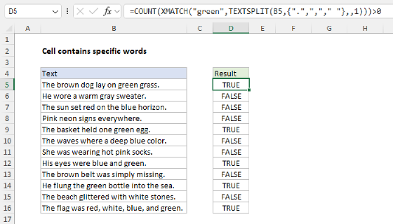
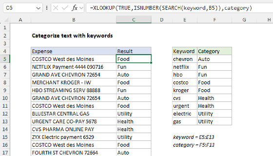
Test for more than one search string
To test a cell for more than one thing (i.e. for one of many substrings), see this example formula.