Explanation
In this example the goal is to return rows in the range B5:E15 that have a specific state value in column E. To make the example dynamic, the state is a variable entered in cell H4. When the state in H4 is changed, the formula should return a new set of records. This is a perfect application for the FILTER function, which is designed to return values that meet specific logical criteria from a set of data.
FILTER function
The FILTER function "filters" a range of data based on supplied criteria. In other words, the FILTER function will extract matching records from a set of data by applying one or more logical tests. The result is an array of matching values from the original data. The FILTER function takes three arguments, and the generic syntax looks like this:
=FILTER(array,include,[if_empty])
In this problem, array is given as B5:E15, which contains the full set of data without headers:
=FILTER(B5:E15,
The include argument is an expression that runs a simple test for matching states:
E5:E15=H4 // test state values
Placing this expression into FILTER as the second argument, we have:
=FILTER(B5:E15,E5:E15=H4,
Finally, the optional if_empty argument is set to "not found" in case no matching data is found:
=FILTER(B5:E15,E5:E15=H4,"not found")
Note the value for if_empty is a text string in double quotes (""). You can customize this message as you like. Supply an empty string ("") to display nothing. If you omit if_empty altogether, FILTER will return a #CALC! error when no data is returned.
When the formula above is entered, the include argument is evaluated. Since there are 11 cells in the range E5:E11 and the value in H4 is "TX", the include expression returns an array of 11 TRUE and FALSE like this:
{TRUE;FALSE;FALSE;TRUE;FALSE;FALSE;FALSE;FALSE;FALSE;TRUE;TRUE}
Notice the TRUE values in this array correspond to records in the data where the State is "TX". This array is used by the FILTER function to retrieve matching data. Only rows where the result is TRUE make it into the final output.
Other fields and criteria
Other fields can be filtered in a similar way. For example, to filter the same data on orders that are greater than $100, you can use FILTER like this:
=FILTER(B5:E15,C5:C15>100,"not found")
You can also configure the logic inside the include argument to apply more complex criteria.
Related formulas

Filter this or that

Filter text contains

Filter exclude blank values
Related functions

FILTER Function
The Excel FILTER function is used to extract matching values from data based on one or more conditions. The output from FILTER is dynamic. If source data or criteria change, FILTER will return a new set of results. This makes FILTER a flexible way to isolate and inspect data without...
Related videos
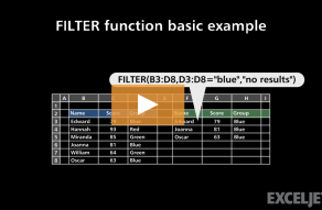
FILTER function basic example